Praxisbeispiel - Telko Kundenabgang-Vorhersage (Telco Customer Churn Prediction) bei Vertragskunden
Die Vorhersage der Kundenabwanderung (bei Vertragssituationen) sagt die Wahrscheinlichkeit voraus, dass Kunden die Produkte oder Dienstleistungen eines Unternehmens kündigen. In den meisten Fällen sind Unternehmen mit Stammkunden oder Kunden im Abonnement bestrebt, ihren Kundenstamm zu erhalten. Daher ist es wichtig, die Kunden zu verfolgen, die ihr Abonnement kündigen, und diejenigen, die den Dienst weiter nutzen. Dieser Ansatz setzt voraus, dass das Unternehmen das Verhalten seiner Kunden kennt und versteht und die Eigenschaften, die zu dem Risiko führen, dass der Kunde das Unternehmen verlässt.
Szenario
Annahme: Wir sind ein Telekommunikations-Unternehmen, das über historische Daten darüber verfügt, wie seine Kunden mit seinen Dienstleistungen interagiert haben. Das Unternehmen möchte wissen, wie hoch die Wahrscheinlichkeit ist, dass Kunden abwandern, damit es gezielte Marketingkampagnen starten kann.
Datensatz
Sage Kundenverhalten voraus, um die Kunden zu binden.
Ihr könnt alle relevanten Kundendaten analysieren und gezielte Kundenbindungsprogramme entwickeln.
https://www.kaggle.com/datasets/blastchar/telco-customer-churn
[1]:
import sys
# !{sys.executable} -m pip install kagglehub
# !{sys.executable} -m pip install @
# !{sys.executable} -m pip install missingno
[2]:
import kagglehub
[3]:
import pandas as pd
import numpy as np
import missingno as msno
import matplotlib.pyplot as plt
import seaborn as sns
import plotly.express as px
import plotly.graph_objects as go
from plotly.subplots import make_subplots
import warnings

pd.set_option("display.max_columns", None)
warnings.filterwarnings("ignore")
[4]:
from sklearn.preprocessing import StandardScaler, LabelEncoder

from sklearn.model_selection import train_test_split

from sklearn.tree import DecisionTreeClassifier
from sklearn.ensemble import RandomForestClassifier
from sklearn.naive_bayes import GaussianNB
from sklearn.neighbors import KNeighborsClassifier
from sklearn.svm import SVC
from sklearn.neural_network import MLPClassifier
from sklearn.ensemble import AdaBoostClassifier
from sklearn.ensemble import GradientBoostingClassifier
from sklearn.ensemble import ExtraTreesClassifier
from sklearn.linear_model import LogisticRegression

from sklearn import metrics
from sklearn.metrics import roc_curve
from sklearn.metrics import accuracy_score, precision_score, recall_score, f1_score, confusion_matrix, classification_report

# from xgboost import XGBClassifier
# from catboost import CatBoostClassifier
[5]:
# Download data from Kaggle
path = kagglehub.dataset_download("blastchar/telco-customer-churn")

print("Path to files:", path)
Path to files: /Users/veit/.cache/kagglehub/datasets/blastchar/telco-customer-churn/versions/1
[6]:
path_file = "~/.cache/kagglehub/datasets/blastchar/telco-customer-churn/versions/1/WA_Fn-UseC_-Telco-Customer-Churn.csv"
print(path_file)
~/.cache/kagglehub/datasets/blastchar/telco-customer-churn/versions/1/WA_Fn-UseC_-Telco-Customer-Churn.csv
Datensatz
[7]:
df = pd.read_csv(path_file)
df
[7]:
| customerID | gender | SeniorCitizen | Partner | Dependents | tenure | PhoneService | MultipleLines | InternetService | OnlineSecurity | OnlineBackup | DeviceProtection | TechSupport | StreamingTV | StreamingMovies | Contract | PaperlessBilling | PaymentMethod | MonthlyCharges | TotalCharges | Churn | |
|---|---|---|---|---|---|---|---|---|---|---|---|---|---|---|---|---|---|---|---|---|---|
| 0 | 7590-VHVEG | Female | 0 | Yes | No | 1 | No | No phone service | DSL | No | Yes | No | No | No | No | Month-to-month | Yes | Electronic check | 29.85 | 29.85 | No |
| 1 | 5575-GNVDE | Male | 0 | No | No | 34 | Yes | No | DSL | Yes | No | Yes | No | No | No | One year | No | Mailed check | 56.95 | 1889.5 | No |
| 2 | 3668-QPYBK | Male | 0 | No | No | 2 | Yes | No | DSL | Yes | Yes | No | No | No | No | Month-to-month | Yes | Mailed check | 53.85 | 108.15 | Yes |
| 3 | 7795-CFOCW | Male | 0 | No | No | 45 | No | No phone service | DSL | Yes | No | Yes | Yes | No | No | One year | No | Bank transfer (automatic) | 42.30 | 1840.75 | No |
| 4 | 9237-HQITU | Female | 0 | No | No | 2 | Yes | No | Fiber optic | No | No | No | No | No | No | Month-to-month | Yes | Electronic check | 70.70 | 151.65 | Yes |
| ... | ... | ... | ... | ... | ... | ... | ... | ... | ... | ... | ... | ... | ... | ... | ... | ... | ... | ... | ... | ... | ... |
| 7038 | 6840-RESVB | Male | 0 | Yes | Yes | 24 | Yes | Yes | DSL | Yes | No | Yes | Yes | Yes | Yes | One year | Yes | Mailed check | 84.80 | 1990.5 | No |
| 7039 | 2234-XADUH | Female | 0 | Yes | Yes | 72 | Yes | Yes | Fiber optic | No | Yes | Yes | No | Yes | Yes | One year | Yes | Credit card (automatic) | 103.20 | 7362.9 | No |
| 7040 | 4801-JZAZL | Female | 0 | Yes | Yes | 11 | No | No phone service | DSL | Yes | No | No | No | No | No | Month-to-month | Yes | Electronic check | 29.60 | 346.45 | No |
| 7041 | 8361-LTMKD | Male | 1 | Yes | No | 4 | Yes | Yes | Fiber optic | No | No | No | No | No | No | Month-to-month | Yes | Mailed check | 74.40 | 306.6 | Yes |
| 7042 | 3186-AJIEK | Male | 0 | No | No | 66 | Yes | No | Fiber optic | Yes | No | Yes | Yes | Yes | Yes | Two year | Yes | Bank transfer (automatic) | 105.65 | 6844.5 | No |
7043 rows × 21 columns
Der Datensatz enthält Informationen über:
ob der Kunde innerhalb des letzten Monats gekündigt hat - Spalte „Churn“
Dienste, für die sich jeder Kunde angemeldet hat - „PhoneService“, „MultipleLines“, „InternetService“, „OnlineSecurity“, „OnlineBackup“, „DeviceProtection“, „TechSupport“ sowie „StreamingTV“ und „StreamingMovies“.
Informationen zum Kundenkonto - „tenure“ wie lange der Kunde bereits Kunde ist, „Contract“ (Vertrag), „PaperlessBilling“ (papierlose Abrechnung), „PaymentMethod“ (Zahlungsmethode), „MonthlyCharges“ (monatliche Gebühren) und „TotalCharges“ (Gesamtgebühren).
Demografische Informationen über Kunden - „gender“ (Geschlecht), „SeniorCitizen“ (Alter) und ob sie „Partner“ (Partner) und „Dependents“ (Familienangehörige) haben.
[8]:
print("shape: ", df.shape)
print()

print(df.info())
shape:  (7043, 21)

<class 'pandas.DataFrame'>
RangeIndex: 7043 entries, 0 to 7042
Data columns (total 21 columns):
 #   Column            Non-Null Count  Dtype
---  ------            --------------  -----
 0   customerID        7043 non-null   str
 1   gender            7043 non-null   str
 2   SeniorCitizen     7043 non-null   int64
 3   Partner           7043 non-null   str
 4   Dependents        7043 non-null   str
 5   tenure            7043 non-null   int64
 6   PhoneService      7043 non-null   str
 7   MultipleLines     7043 non-null   str
 8   InternetService   7043 non-null   str
 9   OnlineSecurity    7043 non-null   str
 10  OnlineBackup      7043 non-null   str
 11  DeviceProtection  7043 non-null   str
 12  TechSupport       7043 non-null   str
 13  StreamingTV       7043 non-null   str
 14  StreamingMovies   7043 non-null   str
 15  Contract          7043 non-null   str
 16  PaperlessBilling  7043 non-null   str
 17  PaymentMethod     7043 non-null   str
 18  MonthlyCharges    7043 non-null   float64
 19  TotalCharges      7043 non-null   str
 20  Churn             7043 non-null   str
dtypes: float64(1), int64(2), str(18)
memory usage: 1.9 MB
None
ACHTUNG!!
Wir sehen, dass „TotalCharges“ hier als object auftaucht, erwarten hier aber einen numerischen Typ. Das muss geändert werden - wir zeigen euch aber erst, was passiert, wenn wir es nicht ändern.
[9]:
df.columns.values
[9]:
<ArrowStringArray>
[      'customerID',           'gender',    'SeniorCitizen',
          'Partner',       'Dependents',           'tenure',
     'PhoneService',    'MultipleLines',  'InternetService',
   'OnlineSecurity',     'OnlineBackup', 'DeviceProtection',
      'TechSupport',      'StreamingTV',  'StreamingMovies',
         'Contract', 'PaperlessBilling',    'PaymentMethod',
   'MonthlyCharges',     'TotalCharges',            'Churn']
Length: 21, dtype: str
[10]:
df.dtypes
[10]:
customerID              str
gender                  str
SeniorCitizen         int64
Partner                 str
Dependents              str
tenure                int64
PhoneService            str
MultipleLines           str
InternetService         str
OnlineSecurity          str
OnlineBackup            str
DeviceProtection        str
TechSupport             str
StreamingTV             str
StreamingMovies         str
Contract                str
PaperlessBilling        str
PaymentMethod           str
MonthlyCharges      float64
TotalCharges            str
Churn                   str
dtype: object
Ermittle fehlende Werte und visualisiere sie
[11]:
## wir kannten schon die isnull() Funktion in pandas

for col in df.columns:
    print(col, df[col].isnull().sum())
customerID 0
gender 0
SeniorCitizen 0
Partner 0
Dependents 0
tenure 0
PhoneService 0
MultipleLines 0
InternetService 0
OnlineSecurity 0
OnlineBackup 0
DeviceProtection 0
TechSupport 0
StreamingTV 0
StreamingMovies 0
Contract 0
PaperlessBilling 0
PaymentMethod 0
MonthlyCharges 0
TotalCharges 0
Churn 0
[12]:
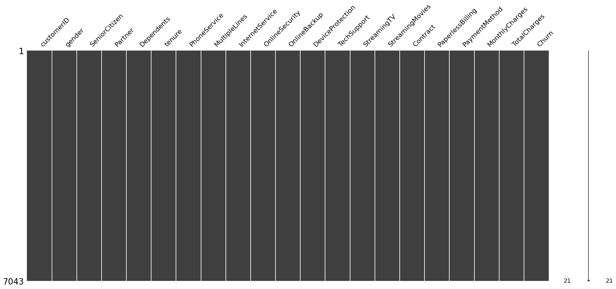
# Zudem könnte man sich die fehlende Werte auch in einer Matrix anzeigen lassen
# (nur haben wir hier keine fehlenden Werte)

msno.matrix(df);
Daten Manipulation / Bereinigung
[13]:
df["TotalCharges"] = pd.to_numeric(df.TotalCharges, errors="coerce")
# print(df.dtypes)
print(df.info())
<class 'pandas.DataFrame'>
RangeIndex: 7043 entries, 0 to 7042
Data columns (total 21 columns):
 #   Column            Non-Null Count  Dtype
---  ------            --------------  -----
 0   customerID        7043 non-null   str
 1   gender            7043 non-null   str
 2   SeniorCitizen     7043 non-null   int64
 3   Partner           7043 non-null   str
 4   Dependents        7043 non-null   str
 5   tenure            7043 non-null   int64
 6   PhoneService      7043 non-null   str
 7   MultipleLines     7043 non-null   str
 8   InternetService   7043 non-null   str
 9   OnlineSecurity    7043 non-null   str
 10  OnlineBackup      7043 non-null   str
 11  DeviceProtection  7043 non-null   str
 12  TechSupport       7043 non-null   str
 13  StreamingTV       7043 non-null   str
 14  StreamingMovies   7043 non-null   str
 15  Contract          7043 non-null   str
 16  PaperlessBilling  7043 non-null   str
 17  PaymentMethod     7043 non-null   str
 18  MonthlyCharges    7043 non-null   float64
 19  TotalCharges      7032 non-null   float64
 20  Churn             7043 non-null   str
dtypes: float64(2), int64(2), str(17)
memory usage: 1.8 MB
None
[14]:
print(df.isnull().sum())
customerID           0
gender               0
SeniorCitizen        0
Partner              0
Dependents           0
tenure               0
PhoneService         0
MultipleLines        0
InternetService      0
OnlineSecurity       0
OnlineBackup         0
DeviceProtection     0
TechSupport          0
StreamingTV          0
StreamingMovies      0
Contract             0
PaperlessBilling     0
PaymentMethod        0
MonthlyCharges       0
TotalCharges        11
Churn                0
dtype: int64
[15]:
# Visualisierung

msno.matrix(df);

[16]:
df[np.isnan(df["TotalCharges"])]
[16]:
| customerID | gender | SeniorCitizen | Partner | Dependents | tenure | PhoneService | MultipleLines | InternetService | OnlineSecurity | OnlineBackup | DeviceProtection | TechSupport | StreamingTV | StreamingMovies | Contract | PaperlessBilling | PaymentMethod | MonthlyCharges | TotalCharges | Churn | |
|---|---|---|---|---|---|---|---|---|---|---|---|---|---|---|---|---|---|---|---|---|---|
| 488 | 4472-LVYGI | Female | 0 | Yes | Yes | 0 | No | No phone service | DSL | Yes | No | Yes | Yes | Yes | No | Two year | Yes | Bank transfer (automatic) | 52.55 | NaN | No |
| 753 | 3115-CZMZD | Male | 0 | No | Yes | 0 | Yes | No | No | No internet service | No internet service | No internet service | No internet service | No internet service | No internet service | Two year | No | Mailed check | 20.25 | NaN | No |
| 936 | 5709-LVOEQ | Female | 0 | Yes | Yes | 0 | Yes | No | DSL | Yes | Yes | Yes | No | Yes | Yes | Two year | No | Mailed check | 80.85 | NaN | No |
| 1082 | 4367-NUYAO | Male | 0 | Yes | Yes | 0 | Yes | Yes | No | No internet service | No internet service | No internet service | No internet service | No internet service | No internet service | Two year | No | Mailed check | 25.75 | NaN | No |
| 1340 | 1371-DWPAZ | Female | 0 | Yes | Yes | 0 | No | No phone service | DSL | Yes | Yes | Yes | Yes | Yes | No | Two year | No | Credit card (automatic) | 56.05 | NaN | No |
| 3331 | 7644-OMVMY | Male | 0 | Yes | Yes | 0 | Yes | No | No | No internet service | No internet service | No internet service | No internet service | No internet service | No internet service | Two year | No | Mailed check | 19.85 | NaN | No |
| 3826 | 3213-VVOLG | Male | 0 | Yes | Yes | 0 | Yes | Yes | No | No internet service | No internet service | No internet service | No internet service | No internet service | No internet service | Two year | No | Mailed check | 25.35 | NaN | No |
| 4380 | 2520-SGTTA | Female | 0 | Yes | Yes | 0 | Yes | No | No | No internet service | No internet service | No internet service | No internet service | No internet service | No internet service | Two year | No | Mailed check | 20.00 | NaN | No |
| 5218 | 2923-ARZLG | Male | 0 | Yes | Yes | 0 | Yes | No | No | No internet service | No internet service | No internet service | No internet service | No internet service | No internet service | One year | Yes | Mailed check | 19.70 | NaN | No |
| 6670 | 4075-WKNIU | Female | 0 | Yes | Yes | 0 | Yes | Yes | DSL | No | Yes | Yes | Yes | Yes | No | Two year | No | Mailed check | 73.35 | NaN | No |
| 6754 | 2775-SEFEE | Male | 0 | No | Yes | 0 | Yes | Yes | DSL | Yes | Yes | No | Yes | No | No | Two year | Yes | Bank transfer (automatic) | 61.90 | NaN | No |
Wir beobachten, dass die Spalte „tenure“ 0 ist bei diesen Einträgen, wo „TotalCharges“ NaN ist, obwohl die Spalte MonthlyCharges nicht leer ist.
Lass uns die Spalte „tenure“ näher anschauen und checken, ob es noch andere 0-Werte in diese Spalte gibt.
[17]:
df[df["tenure"] == 0].index
[17]:
Index([488, 753, 936, 1082, 1340, 3331, 3826, 4380, 5218, 6670, 6754], dtype='int64')
Feststellung und Entscheidung
Der Vergleich zeigt, dass es keine zusätzlichen fehlenden Werte in der „tenure“-Spalte gibt.
Wir löschen die Zeilen mit den fehlenden Werten in „tenure“ und „TotalCharges“, da es nur 11 von 7043 Zeilen sind und wir nicht von gravierenden Konsequenzen durch das Löschen dieser Zeilen ausgehen.
Wenn es nur die fehlenden Werte in „TotalCharges“ wäre, könnte man auch versuchen, die Werte darin durch Extrapolation aufzufüllen mit z.B. mean.
[18]:
# df.drop(df['tenure'] == 0, axis=0, inplace=False)

df_new = df[df["tenure"] != 0]

df_new[df_new['tenure'] == 0].index
[18]:
Index([], dtype='int64')
[19]:
df_new2 = df.drop(labels=df[df['tenure'] == 0].index, axis=0, inplace=False)
df_new2[df_new2['tenure'] == 0].index
[19]:
Index([], dtype='int64')
[20]:
df_new2
[20]:
| customerID | gender | SeniorCitizen | Partner | Dependents | tenure | PhoneService | MultipleLines | InternetService | OnlineSecurity | OnlineBackup | DeviceProtection | TechSupport | StreamingTV | StreamingMovies | Contract | PaperlessBilling | PaymentMethod | MonthlyCharges | TotalCharges | Churn | |
|---|---|---|---|---|---|---|---|---|---|---|---|---|---|---|---|---|---|---|---|---|---|
| 0 | 7590-VHVEG | Female | 0 | Yes | No | 1 | No | No phone service | DSL | No | Yes | No | No | No | No | Month-to-month | Yes | Electronic check | 29.85 | 29.85 | No |
| 1 | 5575-GNVDE | Male | 0 | No | No | 34 | Yes | No | DSL | Yes | No | Yes | No | No | No | One year | No | Mailed check | 56.95 | 1889.50 | No |
| 2 | 3668-QPYBK | Male | 0 | No | No | 2 | Yes | No | DSL | Yes | Yes | No | No | No | No | Month-to-month | Yes | Mailed check | 53.85 | 108.15 | Yes |
| 3 | 7795-CFOCW | Male | 0 | No | No | 45 | No | No phone service | DSL | Yes | No | Yes | Yes | No | No | One year | No | Bank transfer (automatic) | 42.30 | 1840.75 | No |
| 4 | 9237-HQITU | Female | 0 | No | No | 2 | Yes | No | Fiber optic | No | No | No | No | No | No | Month-to-month | Yes | Electronic check | 70.70 | 151.65 | Yes |
| ... | ... | ... | ... | ... | ... | ... | ... | ... | ... | ... | ... | ... | ... | ... | ... | ... | ... | ... | ... | ... | ... |
| 7038 | 6840-RESVB | Male | 0 | Yes | Yes | 24 | Yes | Yes | DSL | Yes | No | Yes | Yes | Yes | Yes | One year | Yes | Mailed check | 84.80 | 1990.50 | No |
| 7039 | 2234-XADUH | Female | 0 | Yes | Yes | 72 | Yes | Yes | Fiber optic | No | Yes | Yes | No | Yes | Yes | One year | Yes | Credit card (automatic) | 103.20 | 7362.90 | No |
| 7040 | 4801-JZAZL | Female | 0 | Yes | Yes | 11 | No | No phone service | DSL | Yes | No | No | No | No | No | Month-to-month | Yes | Electronic check | 29.60 | 346.45 | No |
| 7041 | 8361-LTMKD | Male | 1 | Yes | No | 4 | Yes | Yes | Fiber optic | No | No | No | No | No | No | Month-to-month | Yes | Mailed check | 74.40 | 306.60 | Yes |
| 7042 | 3186-AJIEK | Male | 0 | No | No | 66 | Yes | No | Fiber optic | Yes | No | Yes | Yes | Yes | Yes | Two year | Yes | Bank transfer (automatic) | 105.65 | 6844.50 | No |
7032 rows × 21 columns
[21]:
df[df["tenure"]==0].index
[21]:
Index([488, 753, 936, 1082, 1340, 3331, 3826, 4380, 5218, 6670, 6754], dtype='int64')
[22]:
print(df.shape)
df.drop(labels=df[df["tenure"] == 0].index, axis=0, inplace=True)
df
(7043, 21)
[22]:
| customerID | gender | SeniorCitizen | Partner | Dependents | tenure | PhoneService | MultipleLines | InternetService | OnlineSecurity | OnlineBackup | DeviceProtection | TechSupport | StreamingTV | StreamingMovies | Contract | PaperlessBilling | PaymentMethod | MonthlyCharges | TotalCharges | Churn | |
|---|---|---|---|---|---|---|---|---|---|---|---|---|---|---|---|---|---|---|---|---|---|
| 0 | 7590-VHVEG | Female | 0 | Yes | No | 1 | No | No phone service | DSL | No | Yes | No | No | No | No | Month-to-month | Yes | Electronic check | 29.85 | 29.85 | No |
| 1 | 5575-GNVDE | Male | 0 | No | No | 34 | Yes | No | DSL | Yes | No | Yes | No | No | No | One year | No | Mailed check | 56.95 | 1889.50 | No |
| 2 | 3668-QPYBK | Male | 0 | No | No | 2 | Yes | No | DSL | Yes | Yes | No | No | No | No | Month-to-month | Yes | Mailed check | 53.85 | 108.15 | Yes |
| 3 | 7795-CFOCW | Male | 0 | No | No | 45 | No | No phone service | DSL | Yes | No | Yes | Yes | No | No | One year | No | Bank transfer (automatic) | 42.30 | 1840.75 | No |
| 4 | 9237-HQITU | Female | 0 | No | No | 2 | Yes | No | Fiber optic | No | No | No | No | No | No | Month-to-month | Yes | Electronic check | 70.70 | 151.65 | Yes |
| ... | ... | ... | ... | ... | ... | ... | ... | ... | ... | ... | ... | ... | ... | ... | ... | ... | ... | ... | ... | ... | ... |
| 7038 | 6840-RESVB | Male | 0 | Yes | Yes | 24 | Yes | Yes | DSL | Yes | No | Yes | Yes | Yes | Yes | One year | Yes | Mailed check | 84.80 | 1990.50 | No |
| 7039 | 2234-XADUH | Female | 0 | Yes | Yes | 72 | Yes | Yes | Fiber optic | No | Yes | Yes | No | Yes | Yes | One year | Yes | Credit card (automatic) | 103.20 | 7362.90 | No |
| 7040 | 4801-JZAZL | Female | 0 | Yes | Yes | 11 | No | No phone service | DSL | Yes | No | No | No | No | No | Month-to-month | Yes | Electronic check | 29.60 | 346.45 | No |
| 7041 | 8361-LTMKD | Male | 1 | Yes | No | 4 | Yes | Yes | Fiber optic | No | No | No | No | No | No | Month-to-month | Yes | Mailed check | 74.40 | 306.60 | Yes |
| 7042 | 3186-AJIEK | Male | 0 | No | No | 66 | Yes | No | Fiber optic | Yes | No | Yes | Yes | Yes | Yes | Two year | Yes | Bank transfer (automatic) | 105.65 | 6844.50 | No |
7032 rows × 21 columns
[23]:
df.reset_index()
df
[23]:
| customerID | gender | SeniorCitizen | Partner | Dependents | tenure | PhoneService | MultipleLines | InternetService | OnlineSecurity | OnlineBackup | DeviceProtection | TechSupport | StreamingTV | StreamingMovies | Contract | PaperlessBilling | PaymentMethod | MonthlyCharges | TotalCharges | Churn | |
|---|---|---|---|---|---|---|---|---|---|---|---|---|---|---|---|---|---|---|---|---|---|
| 0 | 7590-VHVEG | Female | 0 | Yes | No | 1 | No | No phone service | DSL | No | Yes | No | No | No | No | Month-to-month | Yes | Electronic check | 29.85 | 29.85 | No |
| 1 | 5575-GNVDE | Male | 0 | No | No | 34 | Yes | No | DSL | Yes | No | Yes | No | No | No | One year | No | Mailed check | 56.95 | 1889.50 | No |
| 2 | 3668-QPYBK | Male | 0 | No | No | 2 | Yes | No | DSL | Yes | Yes | No | No | No | No | Month-to-month | Yes | Mailed check | 53.85 | 108.15 | Yes |
| 3 | 7795-CFOCW | Male | 0 | No | No | 45 | No | No phone service | DSL | Yes | No | Yes | Yes | No | No | One year | No | Bank transfer (automatic) | 42.30 | 1840.75 | No |
| 4 | 9237-HQITU | Female | 0 | No | No | 2 | Yes | No | Fiber optic | No | No | No | No | No | No | Month-to-month | Yes | Electronic check | 70.70 | 151.65 | Yes |
| ... | ... | ... | ... | ... | ... | ... | ... | ... | ... | ... | ... | ... | ... | ... | ... | ... | ... | ... | ... | ... | ... |
| 7038 | 6840-RESVB | Male | 0 | Yes | Yes | 24 | Yes | Yes | DSL | Yes | No | Yes | Yes | Yes | Yes | One year | Yes | Mailed check | 84.80 | 1990.50 | No |
| 7039 | 2234-XADUH | Female | 0 | Yes | Yes | 72 | Yes | Yes | Fiber optic | No | Yes | Yes | No | Yes | Yes | One year | Yes | Credit card (automatic) | 103.20 | 7362.90 | No |
| 7040 | 4801-JZAZL | Female | 0 | Yes | Yes | 11 | No | No phone service | DSL | Yes | No | No | No | No | No | Month-to-month | Yes | Electronic check | 29.60 | 346.45 | No |
| 7041 | 8361-LTMKD | Male | 1 | Yes | No | 4 | Yes | Yes | Fiber optic | No | No | No | No | No | No | Month-to-month | Yes | Mailed check | 74.40 | 306.60 | Yes |
| 7042 | 3186-AJIEK | Male | 0 | No | No | 66 | Yes | No | Fiber optic | Yes | No | Yes | Yes | Yes | Yes | Two year | Yes | Bank transfer (automatic) | 105.65 | 6844.50 | No |
7032 rows × 21 columns
[24]:
df.reset_index(inplace=True)
df
[24]:
| index | customerID | gender | SeniorCitizen | Partner | Dependents | tenure | PhoneService | MultipleLines | InternetService | OnlineSecurity | OnlineBackup | DeviceProtection | TechSupport | StreamingTV | StreamingMovies | Contract | PaperlessBilling | PaymentMethod | MonthlyCharges | TotalCharges | Churn | |
|---|---|---|---|---|---|---|---|---|---|---|---|---|---|---|---|---|---|---|---|---|---|---|
| 0 | 0 | 7590-VHVEG | Female | 0 | Yes | No | 1 | No | No phone service | DSL | No | Yes | No | No | No | No | Month-to-month | Yes | Electronic check | 29.85 | 29.85 | No |
| 1 | 1 | 5575-GNVDE | Male | 0 | No | No | 34 | Yes | No | DSL | Yes | No | Yes | No | No | No | One year | No | Mailed check | 56.95 | 1889.50 | No |
| 2 | 2 | 3668-QPYBK | Male | 0 | No | No | 2 | Yes | No | DSL | Yes | Yes | No | No | No | No | Month-to-month | Yes | Mailed check | 53.85 | 108.15 | Yes |
| 3 | 3 | 7795-CFOCW | Male | 0 | No | No | 45 | No | No phone service | DSL | Yes | No | Yes | Yes | No | No | One year | No | Bank transfer (automatic) | 42.30 | 1840.75 | No |
| 4 | 4 | 9237-HQITU | Female | 0 | No | No | 2 | Yes | No | Fiber optic | No | No | No | No | No | No | Month-to-month | Yes | Electronic check | 70.70 | 151.65 | Yes |
| ... | ... | ... | ... | ... | ... | ... | ... | ... | ... | ... | ... | ... | ... | ... | ... | ... | ... | ... | ... | ... | ... | ... |
| 7027 | 7038 | 6840-RESVB | Male | 0 | Yes | Yes | 24 | Yes | Yes | DSL | Yes | No | Yes | Yes | Yes | Yes | One year | Yes | Mailed check | 84.80 | 1990.50 | No |
| 7028 | 7039 | 2234-XADUH | Female | 0 | Yes | Yes | 72 | Yes | Yes | Fiber optic | No | Yes | Yes | No | Yes | Yes | One year | Yes | Credit card (automatic) | 103.20 | 7362.90 | No |
| 7029 | 7040 | 4801-JZAZL | Female | 0 | Yes | Yes | 11 | No | No phone service | DSL | Yes | No | No | No | No | No | Month-to-month | Yes | Electronic check | 29.60 | 346.45 | No |
| 7030 | 7041 | 8361-LTMKD | Male | 1 | Yes | No | 4 | Yes | Yes | Fiber optic | No | No | No | No | No | No | Month-to-month | Yes | Mailed check | 74.40 | 306.60 | Yes |
| 7031 | 7042 | 3186-AJIEK | Male | 0 | No | No | 66 | Yes | No | Fiber optic | Yes | No | Yes | Yes | Yes | Yes | Two year | Yes | Bank transfer (automatic) | 105.65 | 6844.50 | No |
7032 rows × 22 columns
[25]:
if "index" in df:
    df.drop("index", axis=1, inplace=True)
df
[25]:
| customerID | gender | SeniorCitizen | Partner | Dependents | tenure | PhoneService | MultipleLines | InternetService | OnlineSecurity | OnlineBackup | DeviceProtection | TechSupport | StreamingTV | StreamingMovies | Contract | PaperlessBilling | PaymentMethod | MonthlyCharges | TotalCharges | Churn | |
|---|---|---|---|---|---|---|---|---|---|---|---|---|---|---|---|---|---|---|---|---|---|
| 0 | 7590-VHVEG | Female | 0 | Yes | No | 1 | No | No phone service | DSL | No | Yes | No | No | No | No | Month-to-month | Yes | Electronic check | 29.85 | 29.85 | No |
| 1 | 5575-GNVDE | Male | 0 | No | No | 34 | Yes | No | DSL | Yes | No | Yes | No | No | No | One year | No | Mailed check | 56.95 | 1889.50 | No |
| 2 | 3668-QPYBK | Male | 0 | No | No | 2 | Yes | No | DSL | Yes | Yes | No | No | No | No | Month-to-month | Yes | Mailed check | 53.85 | 108.15 | Yes |
| 3 | 7795-CFOCW | Male | 0 | No | No | 45 | No | No phone service | DSL | Yes | No | Yes | Yes | No | No | One year | No | Bank transfer (automatic) | 42.30 | 1840.75 | No |
| 4 | 9237-HQITU | Female | 0 | No | No | 2 | Yes | No | Fiber optic | No | No | No | No | No | No | Month-to-month | Yes | Electronic check | 70.70 | 151.65 | Yes |
| ... | ... | ... | ... | ... | ... | ... | ... | ... | ... | ... | ... | ... | ... | ... | ... | ... | ... | ... | ... | ... | ... |
| 7027 | 6840-RESVB | Male | 0 | Yes | Yes | 24 | Yes | Yes | DSL | Yes | No | Yes | Yes | Yes | Yes | One year | Yes | Mailed check | 84.80 | 1990.50 | No |
| 7028 | 2234-XADUH | Female | 0 | Yes | Yes | 72 | Yes | Yes | Fiber optic | No | Yes | Yes | No | Yes | Yes | One year | Yes | Credit card (automatic) | 103.20 | 7362.90 | No |
| 7029 | 4801-JZAZL | Female | 0 | Yes | Yes | 11 | No | No phone service | DSL | Yes | No | No | No | No | No | Month-to-month | Yes | Electronic check | 29.60 | 346.45 | No |
| 7030 | 8361-LTMKD | Male | 1 | Yes | No | 4 | Yes | Yes | Fiber optic | No | No | No | No | No | No | Month-to-month | Yes | Mailed check | 74.40 | 306.60 | Yes |
| 7031 | 3186-AJIEK | Male | 0 | No | No | 66 | Yes | No | Fiber optic | Yes | No | Yes | Yes | Yes | Yes | Two year | Yes | Bank transfer (automatic) | 105.65 | 6844.50 | No |
7032 rows × 21 columns
[26]:
df[df["TotalCharges"].isnull()]
[26]:
| customerID | gender | SeniorCitizen | Partner | Dependents | tenure | PhoneService | MultipleLines | InternetService | OnlineSecurity | OnlineBackup | DeviceProtection | TechSupport | StreamingTV | StreamingMovies | Contract | PaperlessBilling | PaymentMethod | MonthlyCharges | TotalCharges | Churn |
|---|
[27]:
df[~df["TotalCharges"].isnull()]
[27]:
| customerID | gender | SeniorCitizen | Partner | Dependents | tenure | PhoneService | MultipleLines | InternetService | OnlineSecurity | OnlineBackup | DeviceProtection | TechSupport | StreamingTV | StreamingMovies | Contract | PaperlessBilling | PaymentMethod | MonthlyCharges | TotalCharges | Churn | |
|---|---|---|---|---|---|---|---|---|---|---|---|---|---|---|---|---|---|---|---|---|---|
| 0 | 7590-VHVEG | Female | 0 | Yes | No | 1 | No | No phone service | DSL | No | Yes | No | No | No | No | Month-to-month | Yes | Electronic check | 29.85 | 29.85 | No |
| 1 | 5575-GNVDE | Male | 0 | No | No | 34 | Yes | No | DSL | Yes | No | Yes | No | No | No | One year | No | Mailed check | 56.95 | 1889.50 | No |
| 2 | 3668-QPYBK | Male | 0 | No | No | 2 | Yes | No | DSL | Yes | Yes | No | No | No | No | Month-to-month | Yes | Mailed check | 53.85 | 108.15 | Yes |
| 3 | 7795-CFOCW | Male | 0 | No | No | 45 | No | No phone service | DSL | Yes | No | Yes | Yes | No | No | One year | No | Bank transfer (automatic) | 42.30 | 1840.75 | No |
| 4 | 9237-HQITU | Female | 0 | No | No | 2 | Yes | No | Fiber optic | No | No | No | No | No | No | Month-to-month | Yes | Electronic check | 70.70 | 151.65 | Yes |
| ... | ... | ... | ... | ... | ... | ... | ... | ... | ... | ... | ... | ... | ... | ... | ... | ... | ... | ... | ... | ... | ... |
| 7027 | 6840-RESVB | Male | 0 | Yes | Yes | 24 | Yes | Yes | DSL | Yes | No | Yes | Yes | Yes | Yes | One year | Yes | Mailed check | 84.80 | 1990.50 | No |
| 7028 | 2234-XADUH | Female | 0 | Yes | Yes | 72 | Yes | Yes | Fiber optic | No | Yes | Yes | No | Yes | Yes | One year | Yes | Credit card (automatic) | 103.20 | 7362.90 | No |
| 7029 | 4801-JZAZL | Female | 0 | Yes | Yes | 11 | No | No phone service | DSL | Yes | No | No | No | No | No | Month-to-month | Yes | Electronic check | 29.60 | 346.45 | No |
| 7030 | 8361-LTMKD | Male | 1 | Yes | No | 4 | Yes | Yes | Fiber optic | No | No | No | No | No | No | Month-to-month | Yes | Mailed check | 74.40 | 306.60 | Yes |
| 7031 | 3186-AJIEK | Male | 0 | No | No | 66 | Yes | No | Fiber optic | Yes | No | Yes | Yes | Yes | Yes | Two year | Yes | Bank transfer (automatic) | 105.65 | 6844.50 | No |
7032 rows × 21 columns
[28]:
df.isnull().sum()
[28]:
customerID          0
gender              0
SeniorCitizen       0
Partner             0
Dependents          0
tenure              0
PhoneService        0
MultipleLines       0
InternetService     0
OnlineSecurity      0
OnlineBackup        0
DeviceProtection    0
TechSupport         0
StreamingTV         0
StreamingMovies     0
Contract            0
PaperlessBilling    0
PaymentMethod       0
MonthlyCharges      0
TotalCharges        0
Churn               0
dtype: int64
EDA - Explorative Data Analysis (Daten Exploration)
[29]:
df["InternetService"].describe()
[29]:
count            7032
unique              3
top       Fiber optic
freq             3096
Name: InternetService, dtype: object
[30]:
df["InternetService"].unique()
[30]:
<ArrowStringArray>
['DSL', 'Fiber optic', 'No']
Length: 3, dtype: str
[31]:
df["InternetService"].value_counts()
[31]:
InternetService
Fiber optic    3096
DSL            2416
No             1520
Name: count, dtype: int64
[32]:
numerical_cols = ["tenure", "MonthlyCharges", "TotalCharges"]
df[numerical_cols].describe()
[32]:
| tenure | MonthlyCharges | TotalCharges | |
|---|---|---|---|
| count | 7032.000000 | 7032.000000 | 7032.000000 |
| mean | 32.421786 | 64.798208 | 2283.300441 |
| std | 24.545260 | 30.085974 | 2266.771362 |
| min | 1.000000 | 18.250000 | 18.800000 |
| 25% | 9.000000 | 35.587500 | 401.450000 |
| 50% | 29.000000 | 70.350000 | 1397.475000 |
| 75% | 55.000000 | 89.862500 | 3794.737500 |
| max | 72.000000 | 118.750000 | 8684.800000 |
[33]:
df["gender"].value_counts()
[33]:
gender
Male      3549
Female    3483
Name: count, dtype: int64
[34]:
df["Churn"].value_counts()
[34]:
Churn
No     5163
Yes    1869
Name: count, dtype: int64
[35]:
# Anzahl der gechurnten Kunden pro Geschlecht ermitteln
print("Churned Customers")
print(df["Churn"][df["Churn"]=="Yes"].groupby(by=df["gender"]).count())
print()
print("Not-yet-churned Customers")
df["Churn"][df["Churn"]=="No"].groupby(by=df["gender"]).count()
Churned Customers
gender
Female    939
Male      930
Name: Churn, dtype: int64

Not-yet-churned Customers
[35]:
gender
Female    2544
Male      2619
Name: Churn, dtype: int64
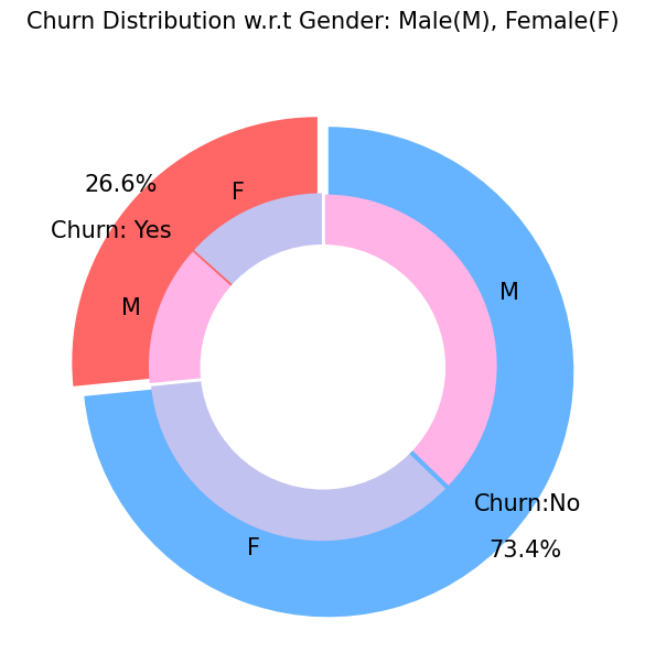
[36]:
## Visualizierung der Churn Verteilung vs. Geschlecht

plt.figure(figsize=(6, 6))
labels =["Churn: Yes","Churn:No"]
values = [1869,5163]
labels_gender = ["F","M","F","M"]
sizes_gender = [939,930 , 2544,2619]
colors = ["#ff6666", "#66b3ff"]
colors_gender = ["#c2c2f0", "#ffb3e6", "#c2c2f0", "#ffb3e6"]
explode = (0.3,0.3)
explode_gender = (0.1,0.1,0.1,0.1)
textprops = {"fontsize":15}
#Plot
plt.pie(values, labels=labels,autopct="%1.1f%%",pctdistance=1.08, labeldistance=0.8,colors=colors, startangle=90,frame=True, explode=explode,radius=10, textprops =textprops, counterclock = True, )
plt.pie(sizes_gender,labels=labels_gender,colors=colors_gender,startangle=90, explode=explode_gender,radius=7, textprops =textprops, counterclock = True, )
#Draw circle
centre_circle = plt.Circle((0,0),5,color="black", fc="white",linewidth=0)
fig = plt.gcf()
fig.gca().add_artist(centre_circle)

plt.title("Churn Distribution w.r.t Gender: Male(M), Female(F)", fontsize=15, y=1.1)

# show plot

plt.axis("equal")
plt.tight_layout()
plt.show()
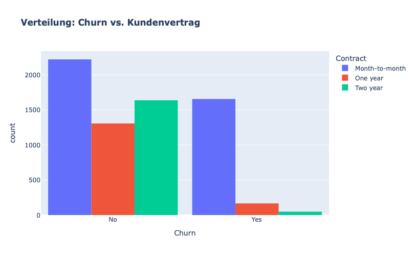
[37]:
## Visualisierung Verteilung: Churn vs. Kundenvertrag

fig = px.histogram(df, x="Churn", color="Contract", barmode="group", title="<b>Verteilung: Churn vs. Kundenvertrag<b>")
fig.update_layout(width=700, height=500, bargap=0.1)
fig.show()
[38]:
# Verteilung: Churn vs. Kunden Zahlungsmethod distribution w.r.t. Churn

fig = px.histogram(df, x="Churn", color="PaymentMethod", title="<b>Verteilung: Churn vs. Kunden Zahlungsmethod distribution w.r.t. Churn</b>")
fig.update_layout(width=700, height=500, bargap=0.1)
fig.show()
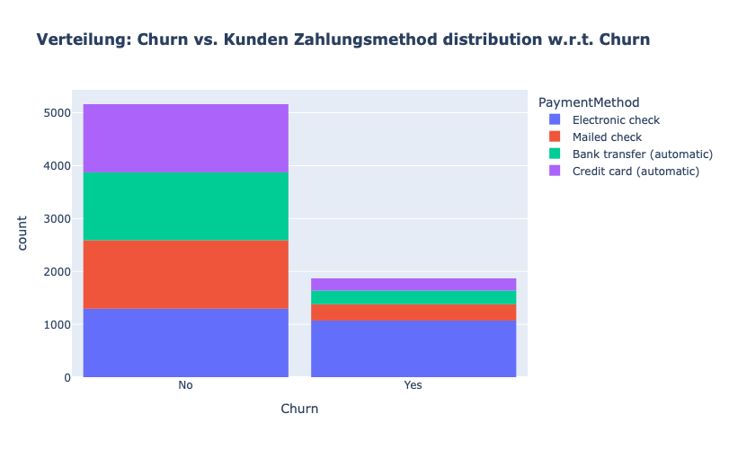
Wir beobachten folgendes:
Die meisten Kunden, die abgewandert sind, hatten einen elektronischen Scheck als Zahlungsmethode.
Kunden, die sich für die automatische Überweisung per Kreditkarte oder Banküberweisung und den Versand von Schecks als Zahlungsmethode entschieden, sind seltener abgewandert.
[39]:
df["InternetService"].unique()
[39]:
<ArrowStringArray>
['DSL', 'Fiber optic', 'No']
Length: 3, dtype: str
[40]:
df[df["gender"]=="Male"][["InternetService", "Churn"]].value_counts()
[40]:
InternetService  Churn
DSL              No       992
Fiber optic      No       910
No               No       717
Fiber optic      Yes      633
DSL              Yes      240
No               Yes       57
Name: count, dtype: int64
[41]:
df[df["gender"]=="Female"][["InternetService", "Churn"]].value_counts()
[41]:
InternetService  Churn
DSL              No       965
Fiber optic      No       889
No               No       690
Fiber optic      Yes      664
DSL              Yes      219
No               Yes       56
Name: count, dtype: int64
[42]:
fig = go.Figure()

fig.add_trace(go.Bar(
  x = [["Churn:No", "Churn:No", "Churn:Yes", "Churn:Yes"],
       ["Female", "Male", "Female", "Male"]],
  y = [965, 992, 219, 240],
  name = 'DSL',
))

fig.add_trace(go.Bar(
  x = [["Churn:No", "Churn:No", "Churn:Yes", "Churn:Yes"],
       ["Female", "Male", "Female", "Male"]],
  y = [889, 910, 664, 633],
  name = "Fiber optic",
))

fig.add_trace(go.Bar(
  x = [["Churn:No", "Churn:No", "Churn:Yes", "Churn:Yes"],
       ["Female", "Male", "Female", "Male"]],
  y = [690, 717, 56, 57],
  name = "No Internet",
))

fig.update_layout(title_text="<b>Verteilung: Churn vs. InternetService und Geschlecht</b>")

fig.show()
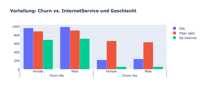
Viele Kunden hatten sich für den Glasfaserdienst (Fiber optic) entschieden. Diese scheinen eine hohe Abwanderungsrate zu haben, was auf eine Unzufriedenheit mit dieser Art von Internetdienst hindeuten könnte.
Kunden, die einen DSL-Dienst nutzen, sind in der Mehrzahl und haben eine geringere Abwanderungsrate als Glasfaserkunden.
[43]:
color_map = {"Yes": "#FF97FF", "No": "#AB63FA"}
fig = px.histogram(df, x="Churn", color="Dependents", barmode="group", title="<b>Verteilung: Churn vs. Familienangehörige</b>", color_discrete_map=color_map)
fig.update_layout(width=700, height=500, bargap=0.1)
fig.show()
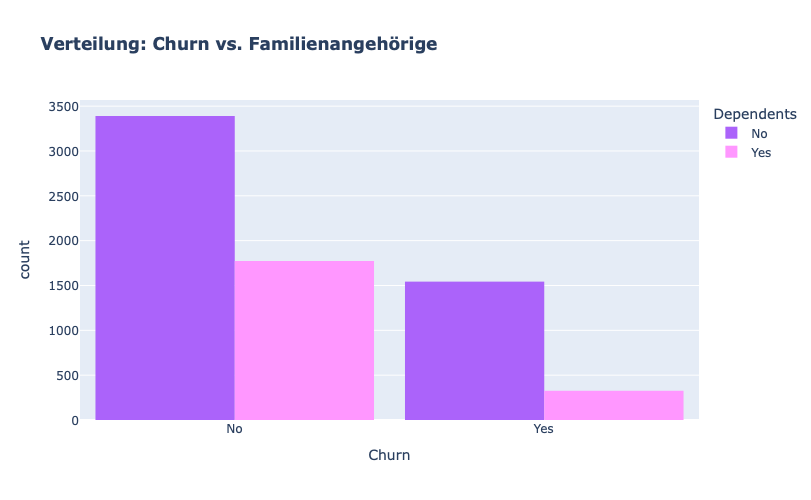
Es scheint, dass die Kunden ohne Familienangehörige („dependents“) wahrscheinlicher abwandern.
[44]:
color_map = {"Yes": '#FFA15A', "No": '#00CC96'}
fig = px.histogram(df, x="Churn", color="Partner", barmode="group", title="<b>Verteilung: Churn vs. Partners</b>", color_discrete_map=color_map)
fig.update_layout(width=700, height=500, bargap=0.1)
fig.show()
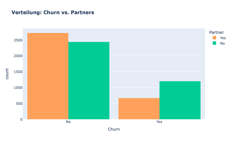
Kunden OHNE Partner scheinen eher dazu zu tendieren abzuwandern.
[45]:
color_map = {"Yes": "#00CC96", "No": "#B6E880"}
fig = px.histogram(df, x="Churn", color="SeniorCitizen", title="<b>Verteilung: Churn vs. Senior Citizen</b>", color_discrete_map=color_map)
fig.update_layout(width=700, height=500, bargap=0.1)
fig.show()
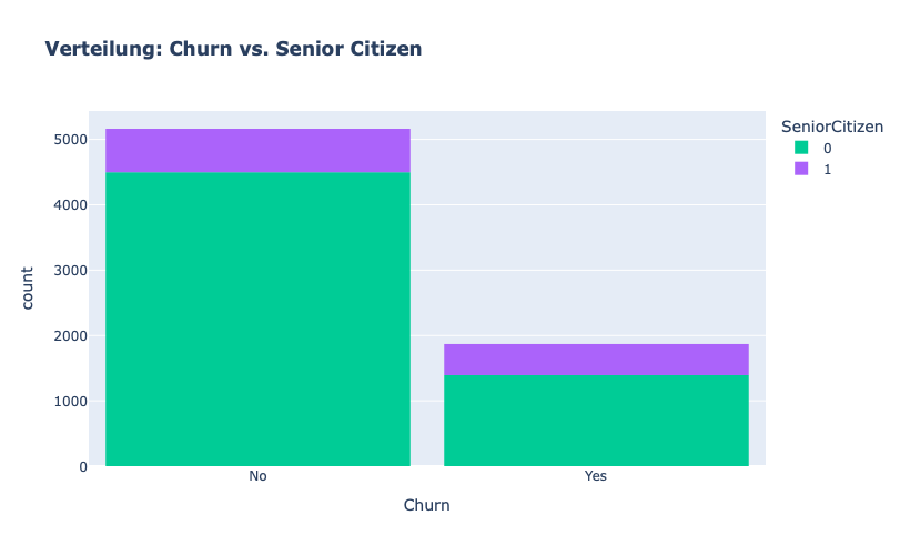
Wir stellen fest, dass generell der Anteil an „seniorigen“ Kunden recht niedrig ist.
Dazu kann man sagen, dass ein die seniorigen Kunden eher dazu tendieren abzuwandern.
[46]:
color_map = {"Yes": "#FF97FF", "No": "#AB63FA"}
fig = px.histogram(df, x="Churn", color="OnlineSecurity", barmode="group", title="<b>Verteilung: Churn vs. Online Security</b>", color_discrete_map=color_map)
fig.update_layout(width=700, height=500, bargap=0.1)
fig.show()
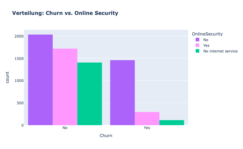
Kunden OHNE Online Security tendieren stark dazu abzuwandern.
[47]:
color_map = {"Yes": "#FFA15A", "No": "#00CC96"}
fig = px.histogram(df, x="Churn", color="PaperlessBilling",  title="<b>Verteilung: Churn vs. Papierlose Rechnung</b>", color_discrete_map=color_map)
fig.update_layout(width=700, height=500, bargap=0.1)
fig.show()
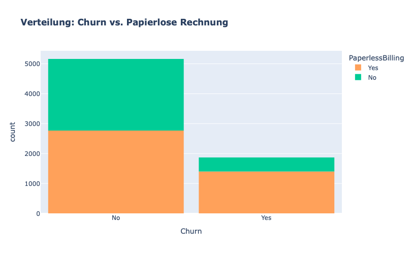
Kunden mit Papierlosen Zahlen scheinen dazu zu tendieren, abzuwandern.
[48]:
fig = px.histogram(df, x="Churn", color="TechSupport",barmode="group",  title="<b>Verteilung: Churn vs. TechSupport</b>")
fig.update_layout(width=700, height=500, bargap=0.1)
fig.show()
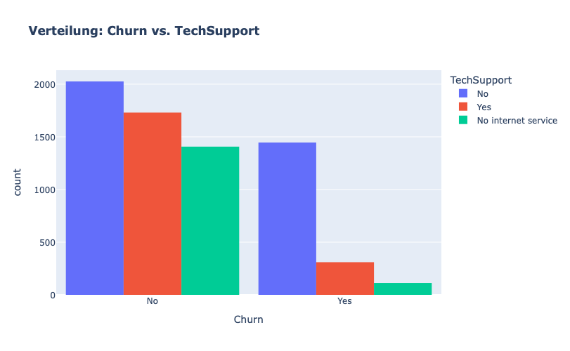
Kunden OHNE TechSupport scheinen stark dazu zu tendieren abzuwandern
[49]:
sns.set_context("paper",font_scale=1.1)
ax = sns.kdeplot(df.MonthlyCharges[(df["Churn"] == "No") ],
                color="Red", shade = True);
ax = sns.kdeplot(df.MonthlyCharges[(df["Churn"] == "Yes") ],
                ax =ax, color="Blue", shade= True);
ax.legend(["Not Churn","Churn"],loc='upper right');
ax.set_ylabel("Density");
ax.set_xlabel("Monthly Charges");
ax.set_title("Verteilung: Churn vs. Monthly Charges");
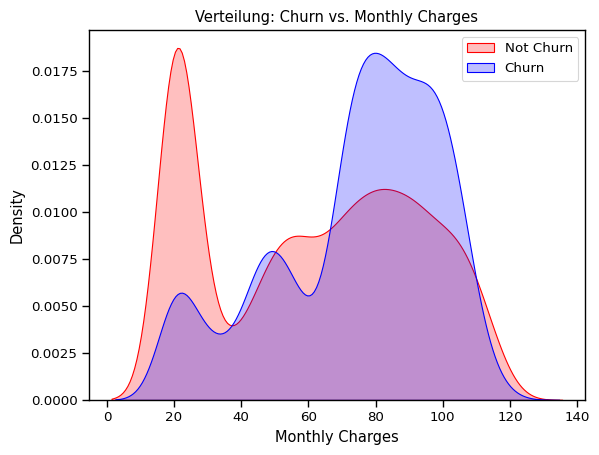
Kunden MIT höheren monatlichen Kosten tendieren eher dazu abzuwandern
[50]:
ax = sns.kdeplot(df.TotalCharges[(df["Churn"] == "No") ],
                color="Gold", shade = True);
ax = sns.kdeplot(df.TotalCharges[(df["Churn"] == "Yes") ],
                ax =ax, color="Green", shade= True);
ax.legend(["Not Chu0rn","Churn"],loc="upper right");
ax.set_ylabel("Density");
ax.set_xlabel("Total Charges");
ax.set_title("Verteilung: Churn vs. Total Charges");
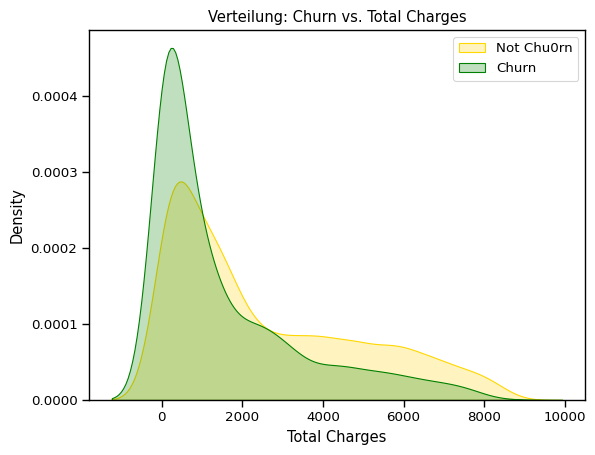
Interessanterweise scheint der höhere Total Charge keine direkte Auswirkung auf erhöhte Abwanderungwahrscheinlichkeit zu haben.
[51]:
fig = px.box(df, x="Churn", y = "tenure")

# Update yaxis properties
fig.update_yaxes(title_text="Tenure (Months)", row=1, col=1)
# Update xaxis properties
fig.update_xaxes(title_text="Churn", row=1, col=1)

# Update size and title
fig.update_layout(autosize=True, width=750, height=600,
    title_font=dict(size=25, family="Courier"),
    title="<b>Tenure vs Churn</b>",
)

fig.show()
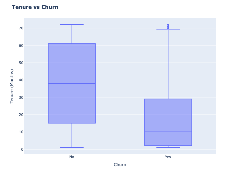
NEUE Kunden scheinen tendenziell eher abzuwandern.
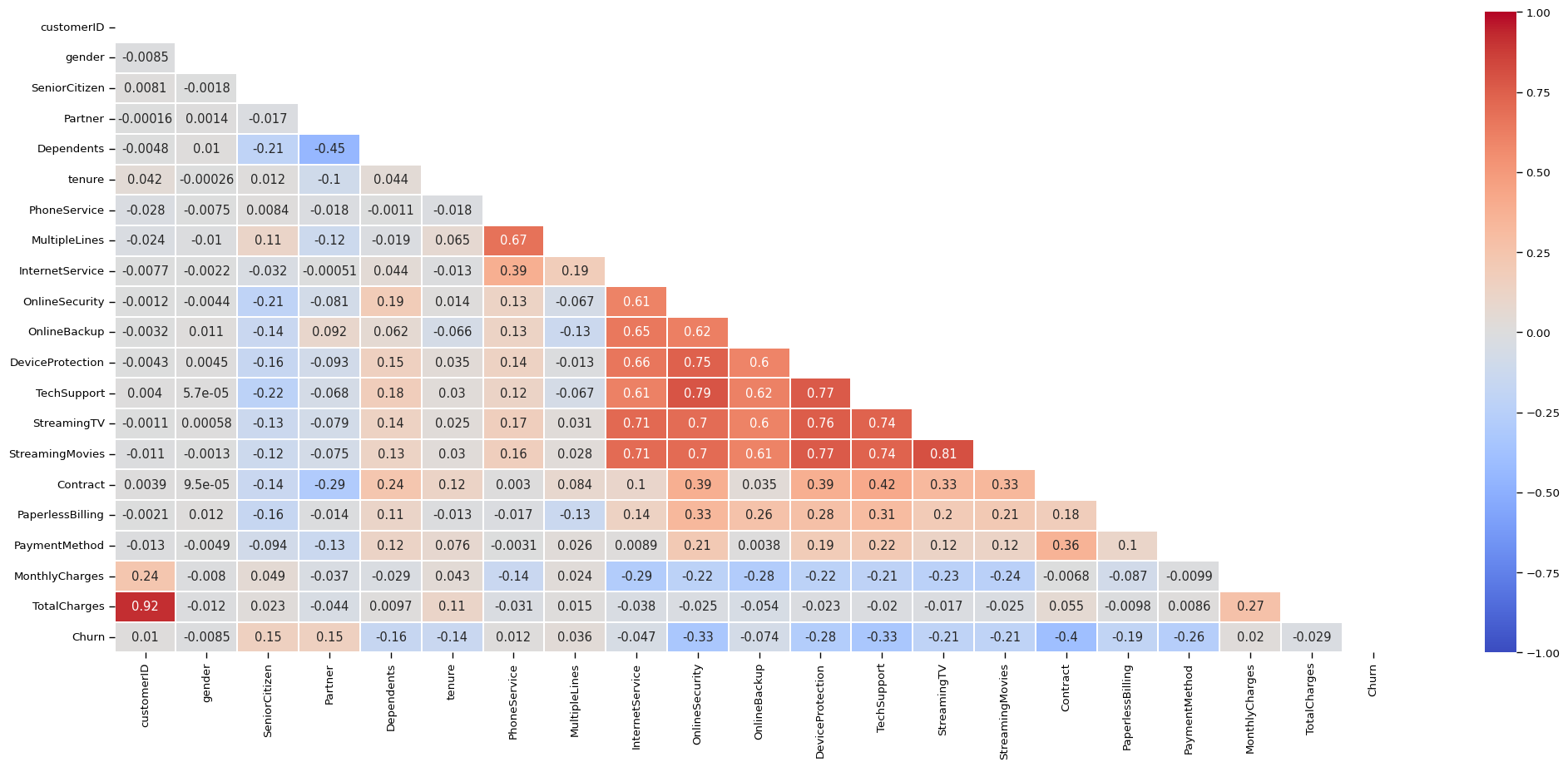
[52]:
# Plotte den Correlation Heatmap (pandas nutzt Pearson Correlation by default)

plt.figure(figsize=(25, 10))

corr = df.apply(lambda x: pd.factorize(x)[0]).corr()

mask = np.triu(np.ones_like(corr, dtype=bool))

ax = sns.heatmap(corr, mask=mask, xticklabels=corr.columns, yticklabels=corr.columns, annot=True, linewidths=.2, cmap="coolwarm", vmin=-1, vmax=1)
[53]:
df.OnlineSecurity.value_counts()
[53]:
OnlineSecurity
No                     3497
Yes                    2015
No internet service    1520
Name: count, dtype: int64
Data Preprocessing
Zielvariable CHURN
Da es sich um ein binäres Klassifikationsproblem hanaelt, sollte die Target-Variable eine binäre Variable sein (numerisch ausgedrückt). Da sie aktuell noch nur String ist, wird nun die Churn-Spalte als Erstes in binary umgewandelt.
[54]:
df["Churn"] = df["Churn"].map({"Yes": 1, "No": 0})

df.head()
[54]:
| customerID | gender | SeniorCitizen | Partner | Dependents | tenure | PhoneService | MultipleLines | InternetService | OnlineSecurity | OnlineBackup | DeviceProtection | TechSupport | StreamingTV | StreamingMovies | Contract | PaperlessBilling | PaymentMethod | MonthlyCharges | TotalCharges | Churn | |
|---|---|---|---|---|---|---|---|---|---|---|---|---|---|---|---|---|---|---|---|---|---|
| 0 | 7590-VHVEG | Female | 0 | Yes | No | 1 | No | No phone service | DSL | No | Yes | No | No | No | No | Month-to-month | Yes | Electronic check | 29.85 | 29.85 | 0 |
| 1 | 5575-GNVDE | Male | 0 | No | No | 34 | Yes | No | DSL | Yes | No | Yes | No | No | No | One year | No | Mailed check | 56.95 | 1889.50 | 0 |
| 2 | 3668-QPYBK | Male | 0 | No | No | 2 | Yes | No | DSL | Yes | Yes | No | No | No | No | Month-to-month | Yes | Mailed check | 53.85 | 108.15 | 1 |
| 3 | 7795-CFOCW | Male | 0 | No | No | 45 | No | No phone service | DSL | Yes | No | Yes | Yes | No | No | One year | No | Bank transfer (automatic) | 42.30 | 1840.75 | 0 |
| 4 | 9237-HQITU | Female | 0 | No | No | 2 | Yes | No | Fiber optic | No | No | No | No | No | No | Month-to-month | Yes | Electronic check | 70.70 | 151.65 | 1 |
Wir entfernen die customerID-Spalte.
[55]:
## Verwerfe ID-columns
if "customerID" in df:
    df.drop("customerID", axis=1, inplace=True)

df
[55]:
| gender | SeniorCitizen | Partner | Dependents | tenure | PhoneService | MultipleLines | InternetService | OnlineSecurity | OnlineBackup | DeviceProtection | TechSupport | StreamingTV | StreamingMovies | Contract | PaperlessBilling | PaymentMethod | MonthlyCharges | TotalCharges | Churn | |
|---|---|---|---|---|---|---|---|---|---|---|---|---|---|---|---|---|---|---|---|---|
| 0 | Female | 0 | Yes | No | 1 | No | No phone service | DSL | No | Yes | No | No | No | No | Month-to-month | Yes | Electronic check | 29.85 | 29.85 | 0 |
| 1 | Male | 0 | No | No | 34 | Yes | No | DSL | Yes | No | Yes | No | No | No | One year | No | Mailed check | 56.95 | 1889.50 | 0 |
| 2 | Male | 0 | No | No | 2 | Yes | No | DSL | Yes | Yes | No | No | No | No | Month-to-month | Yes | Mailed check | 53.85 | 108.15 | 1 |
| 3 | Male | 0 | No | No | 45 | No | No phone service | DSL | Yes | No | Yes | Yes | No | No | One year | No | Bank transfer (automatic) | 42.30 | 1840.75 | 0 |
| 4 | Female | 0 | No | No | 2 | Yes | No | Fiber optic | No | No | No | No | No | No | Month-to-month | Yes | Electronic check | 70.70 | 151.65 | 1 |
| ... | ... | ... | ... | ... | ... | ... | ... | ... | ... | ... | ... | ... | ... | ... | ... | ... | ... | ... | ... | ... |
| 7027 | Male | 0 | Yes | Yes | 24 | Yes | Yes | DSL | Yes | No | Yes | Yes | Yes | Yes | One year | Yes | Mailed check | 84.80 | 1990.50 | 0 |
| 7028 | Female | 0 | Yes | Yes | 72 | Yes | Yes | Fiber optic | No | Yes | Yes | No | Yes | Yes | One year | Yes | Credit card (automatic) | 103.20 | 7362.90 | 0 |
| 7029 | Female | 0 | Yes | Yes | 11 | No | No phone service | DSL | Yes | No | No | No | No | No | Month-to-month | Yes | Electronic check | 29.60 | 346.45 | 0 |
| 7030 | Male | 1 | Yes | No | 4 | Yes | Yes | Fiber optic | No | No | No | No | No | No | Month-to-month | Yes | Mailed check | 74.40 | 306.60 | 1 |
| 7031 | Male | 0 | No | No | 66 | Yes | No | Fiber optic | Yes | No | Yes | Yes | Yes | Yes | Two year | Yes | Bank transfer (automatic) | 105.65 | 6844.50 | 0 |
7032 rows × 20 columns
Nun haben wir uns schon sehr vieles angeschaut und viel getan …
Muessten wir noch etwas tun, bevor wir die Daten splitten? Können wir den Datensatz nun direkt dem Modell zuführen?
Kategorische Spalten umwandeln
Um die kategorischen Spalten richtig in numerische Spalten umzuwandeln, lass uns sie genauer anschauen und identifizieren, was sich hinter den Strings wirklich verbirgt.
[56]:
df
[56]:
| gender | SeniorCitizen | Partner | Dependents | tenure | PhoneService | MultipleLines | InternetService | OnlineSecurity | OnlineBackup | DeviceProtection | TechSupport | StreamingTV | StreamingMovies | Contract | PaperlessBilling | PaymentMethod | MonthlyCharges | TotalCharges | Churn | |
|---|---|---|---|---|---|---|---|---|---|---|---|---|---|---|---|---|---|---|---|---|
| 0 | Female | 0 | Yes | No | 1 | No | No phone service | DSL | No | Yes | No | No | No | No | Month-to-month | Yes | Electronic check | 29.85 | 29.85 | 0 |
| 1 | Male | 0 | No | No | 34 | Yes | No | DSL | Yes | No | Yes | No | No | No | One year | No | Mailed check | 56.95 | 1889.50 | 0 |
| 2 | Male | 0 | No | No | 2 | Yes | No | DSL | Yes | Yes | No | No | No | No | Month-to-month | Yes | Mailed check | 53.85 | 108.15 | 1 |
| 3 | Male | 0 | No | No | 45 | No | No phone service | DSL | Yes | No | Yes | Yes | No | No | One year | No | Bank transfer (automatic) | 42.30 | 1840.75 | 0 |
| 4 | Female | 0 | No | No | 2 | Yes | No | Fiber optic | No | No | No | No | No | No | Month-to-month | Yes | Electronic check | 70.70 | 151.65 | 1 |
| ... | ... | ... | ... | ... | ... | ... | ... | ... | ... | ... | ... | ... | ... | ... | ... | ... | ... | ... | ... | ... |
| 7027 | Male | 0 | Yes | Yes | 24 | Yes | Yes | DSL | Yes | No | Yes | Yes | Yes | Yes | One year | Yes | Mailed check | 84.80 | 1990.50 | 0 |
| 7028 | Female | 0 | Yes | Yes | 72 | Yes | Yes | Fiber optic | No | Yes | Yes | No | Yes | Yes | One year | Yes | Credit card (automatic) | 103.20 | 7362.90 | 0 |
| 7029 | Female | 0 | Yes | Yes | 11 | No | No phone service | DSL | Yes | No | No | No | No | No | Month-to-month | Yes | Electronic check | 29.60 | 346.45 | 0 |
| 7030 | Male | 1 | Yes | No | 4 | Yes | Yes | Fiber optic | No | No | No | No | No | No | Month-to-month | Yes | Mailed check | 74.40 | 306.60 | 1 |
| 7031 | Male | 0 | No | No | 66 | Yes | No | Fiber optic | Yes | No | Yes | Yes | Yes | Yes | Two year | Yes | Bank transfer (automatic) | 105.65 | 6844.50 | 0 |
7032 rows × 20 columns
DatenAnalyse:
Ist die Spalte:
binary?
boolean?
categorical?
numeric?
Datentypen und ihre Spalten:
binary: gender;
boolean: SeniorCitizen(*), Partner, Dependents, PhoneService, OnlineSecurity, OnlineBackup, DeviceProtection, TechSupport, StreamingTV, StreamingMovies, PaperlessBilling
categorical: MultipleLines, InternetService, Contract, PaymentMethod
numeric: tenure, MonthlyCharges, TotalCharges
(*)SeniorCitizen: In diesem Datensatz ist die Spalte bereits durch 0 und 1 ausgedrückt, d.h. rein rechnerisch bräuchte sie nicht nochmal extra als boolean aufgenommen werden. Allerdings sorgt es für mehr Robustheit und Stabilität in der Pipeline und somit Best Practice, doch alle Datentypen entsprechend zu identifizieren.
Recap:
OrdinalEncoder: gut für kategorische Werte, die eine innere Ordnung bzw Rang haben, z.B. „niedrig“, „medium“, „hoch“ in Umfrageantworte
OneHotEncoder: gut für kategorische Features ohne bestimmte innere Ordnung in einem „one-hot numerischen Array“.
Achtung: OneHotEncoder kann die Dimension (Anzahl Spalten) der Feature-Matrix drastisch erhöhen und „spärliche Matrizen“ (scarce matrices) mit lauter „0“ in der Spalte kreieren, wenn die Originalspalte viele verschieden Werte hat (hohe Kardinalität), was wiederum schlechte Datenqualität bedeuten würde. Alternativen: Es gibt auch weitere Alternativen zum One-Hot-Encoding, z.B. kann man auf Frequency (Count) Encoding ausweichen:
hier werden Kategorien basierend auf der Frequency (Häufigkeit, in denen sie auftreten) im Datensatz. Das kann helfen, die Wichtigkeit dieser Kategorie im Datensatz direkt zu erfassen und mitzugeben. Hat aber auch Pitfalls, z.B. wenn das ein biased Datensatz ist.
Achtung!!
Label-Encoder (in scikit-learn: https://scikit-learn.org/stable/modules/generated/sklearn.preprocessing.LabelEncoder.html):
transformiert die ZIELVARIABLE in integers von 0 bis n-1 (n=Anzahl Klassen), gut geeignet bei „gleichwertigen“ Klassen
Unterteile die Columns in 3 Kategorien: Standardisierung, Ordinal-Encoding and One-Hot-Encoding
binary (direkte Umwandlung zu 0-1): gender
boolean (direkte Umwandlung zu 0-1): SeniorCitizen, Partner, Dependents, PhoneService, OnlineSecurity, OnlineBackup, DeviceProtection, TechSupport, StreamingTV, StreamingMovies, PaperlessBilling
categorical (One-Hot oder Frequency Encoding etc): MultipleLines, InternetService, Contract, PaymentMethod
numeric: tenure, MonthlyCharges, TotalCharges
[57]:
cols_binary = ["gender"]
cols_boolean = ["SeniorCitizen", "Partner", "Dependents", "PhoneService", "OnlineSecurity", "OnlineBackup",
               "DeviceProtection", "TechSupport", "StreamingTV", "StreamingMovies", "PaperlessBilling"]
cols_cat = ["MultipleLines", "InternetService", "Contract", "PaymentMethod"]
cols_numeric = ["tenure", "MonthlyCharges", "TotalCharges"]
[58]:
df[cols_boolean]
[58]:
| SeniorCitizen | Partner | Dependents | PhoneService | OnlineSecurity | OnlineBackup | DeviceProtection | TechSupport | StreamingTV | StreamingMovies | PaperlessBilling | |
|---|---|---|---|---|---|---|---|---|---|---|---|
| 0 | 0 | Yes | No | No | No | Yes | No | No | No | No | Yes |
| 1 | 0 | No | No | Yes | Yes | No | Yes | No | No | No | No |
| 2 | 0 | No | No | Yes | Yes | Yes | No | No | No | No | Yes |
| 3 | 0 | No | No | No | Yes | No | Yes | Yes | No | No | No |
| 4 | 0 | No | No | Yes | No | No | No | No | No | No | Yes |
| ... | ... | ... | ... | ... | ... | ... | ... | ... | ... | ... | ... |
| 7027 | 0 | Yes | Yes | Yes | Yes | No | Yes | Yes | Yes | Yes | Yes |
| 7028 | 0 | Yes | Yes | Yes | No | Yes | Yes | No | Yes | Yes | Yes |
| 7029 | 0 | Yes | Yes | No | Yes | No | No | No | No | No | Yes |
| 7030 | 1 | Yes | No | Yes | No | No | No | No | No | No | Yes |
| 7031 | 0 | No | No | Yes | Yes | No | Yes | Yes | Yes | Yes | Yes |
7032 rows × 11 columns
[59]:
df[cols_cat]
[59]:
| MultipleLines | InternetService | Contract | PaymentMethod | |
|---|---|---|---|---|
| 0 | No phone service | DSL | Month-to-month | Electronic check |
| 1 | No | DSL | One year | Mailed check |
| 2 | No | DSL | Month-to-month | Mailed check |
| 3 | No phone service | DSL | One year | Bank transfer (automatic) |
| 4 | No | Fiber optic | Month-to-month | Electronic check |
| ... | ... | ... | ... | ... |
| 7027 | Yes | DSL | One year | Mailed check |
| 7028 | Yes | Fiber optic | One year | Credit card (automatic) |
| 7029 | No phone service | DSL | Month-to-month | Electronic check |
| 7030 | Yes | Fiber optic | Month-to-month | Mailed check |
| 7031 | No | Fiber optic | Two year | Bank transfer (automatic) |
7032 rows × 4 columns
[60]:
# Mapping von "Female" zu 1 und "Male" zu 0

df["gender"] = df["gender"].map({"Female": 1, "Male": 0})
df["gender"]
[60]:
0       1
1       0
2       0
3       0
4       1
       ..
7027    0
7028    1
7029    1
7030    0
7031    0
Name: gender, Length: 7032, dtype: int64
[61]:
cols_boolean
[61]:
['SeniorCitizen',
 'Partner',
 'Dependents',
 'PhoneService',
 'OnlineSecurity',
 'OnlineBackup',
 'DeviceProtection',
 'TechSupport',
 'StreamingTV',
 'StreamingMovies',
 'PaperlessBilling']
One-Hot-Encoding Spalten mit Werten auffüllen.
Von den original-kartegorischen Spaltenwerten zu den neuen Werten in den neuen One-Hot-Encoded Spalten:
Wir erinnern uns: Ziel liegt darin, die die Spalten mit dem Textwert ‚yes‘ / ‚no‘ in numerische Binärwerte umzuwandeln
eq("yes"):vergleicht elementweise: Ist der Wert in der Spalte gleich
"yes"?Ergebnis ist eine Boolean-Serie: True für
"yes", False für"no".falls Spalte bereits als boolean vorliegt, bräuchte man das ggf nicht, da direkt multipliziert werden kann.
mul(1)elementweise Multiplikation und mappt Booleans zu Zahlen (True wird intern als 1 interpretiert und False als 0), daher wird
True * 1 => 1undFalse * 1 => 0. Somit wird aus ‚yes/no‘ effektiv 1/0.
=> d.h. man könnte auch df[col].map({"yes":1,"no":0}) nutzen anstatt df[col].eq("yes").mul(1).
[62]:
for col in cols_boolean:
    df[col] = df[col].eq("yes").mul(1)

df[cols_boolean]
[62]:
| SeniorCitizen | Partner | Dependents | PhoneService | OnlineSecurity | OnlineBackup | DeviceProtection | TechSupport | StreamingTV | StreamingMovies | PaperlessBilling | |
|---|---|---|---|---|---|---|---|---|---|---|---|
| 0 | 0 | 0 | 0 | 0 | 0 | 0 | 0 | 0 | 0 | 0 | 0 |
| 1 | 0 | 0 | 0 | 0 | 0 | 0 | 0 | 0 | 0 | 0 | 0 |
| 2 | 0 | 0 | 0 | 0 | 0 | 0 | 0 | 0 | 0 | 0 | 0 |
| 3 | 0 | 0 | 0 | 0 | 0 | 0 | 0 | 0 | 0 | 0 | 0 |
| 4 | 0 | 0 | 0 | 0 | 0 | 0 | 0 | 0 | 0 | 0 | 0 |
| ... | ... | ... | ... | ... | ... | ... | ... | ... | ... | ... | ... |
| 7027 | 0 | 0 | 0 | 0 | 0 | 0 | 0 | 0 | 0 | 0 | 0 |
| 7028 | 0 | 0 | 0 | 0 | 0 | 0 | 0 | 0 | 0 | 0 | 0 |
| 7029 | 0 | 0 | 0 | 0 | 0 | 0 | 0 | 0 | 0 | 0 | 0 |
| 7030 | 0 | 0 | 0 | 0 | 0 | 0 | 0 | 0 | 0 | 0 | 0 |
| 7031 | 0 | 0 | 0 | 0 | 0 | 0 | 0 | 0 | 0 | 0 | 0 |
7032 rows × 11 columns
[63]:
# One-Hot-Encoding für die drei kategorischen Spalten

df_onehot_encoded = pd.get_dummies(df, columns=cols_cat) # dtype=int

print(df_onehot_encoded.shape)
df_onehot_encoded
(7032, 29)
[63]:
| gender | SeniorCitizen | Partner | Dependents | tenure | PhoneService | OnlineSecurity | OnlineBackup | DeviceProtection | TechSupport | StreamingTV | StreamingMovies | PaperlessBilling | MonthlyCharges | TotalCharges | Churn | MultipleLines_No | MultipleLines_No phone service | MultipleLines_Yes | InternetService_DSL | InternetService_Fiber optic | InternetService_No | Contract_Month-to-month | Contract_One year | Contract_Two year | PaymentMethod_Bank transfer (automatic) | PaymentMethod_Credit card (automatic) | PaymentMethod_Electronic check | PaymentMethod_Mailed check | |
|---|---|---|---|---|---|---|---|---|---|---|---|---|---|---|---|---|---|---|---|---|---|---|---|---|---|---|---|---|---|
| 0 | 1 | 0 | 0 | 0 | 1 | 0 | 0 | 0 | 0 | 0 | 0 | 0 | 0 | 29.85 | 29.85 | 0 | False | True | False | True | False | False | True | False | False | False | False | True | False |
| 1 | 0 | 0 | 0 | 0 | 34 | 0 | 0 | 0 | 0 | 0 | 0 | 0 | 0 | 56.95 | 1889.50 | 0 | True | False | False | True | False | False | False | True | False | False | False | False | True |
| 2 | 0 | 0 | 0 | 0 | 2 | 0 | 0 | 0 | 0 | 0 | 0 | 0 | 0 | 53.85 | 108.15 | 1 | True | False | False | True | False | False | True | False | False | False | False | False | True |
| 3 | 0 | 0 | 0 | 0 | 45 | 0 | 0 | 0 | 0 | 0 | 0 | 0 | 0 | 42.30 | 1840.75 | 0 | False | True | False | True | False | False | False | True | False | True | False | False | False |
| 4 | 1 | 0 | 0 | 0 | 2 | 0 | 0 | 0 | 0 | 0 | 0 | 0 | 0 | 70.70 | 151.65 | 1 | True | False | False | False | True | False | True | False | False | False | False | True | False |
| ... | ... | ... | ... | ... | ... | ... | ... | ... | ... | ... | ... | ... | ... | ... | ... | ... | ... | ... | ... | ... | ... | ... | ... | ... | ... | ... | ... | ... | ... |
| 7027 | 0 | 0 | 0 | 0 | 24 | 0 | 0 | 0 | 0 | 0 | 0 | 0 | 0 | 84.80 | 1990.50 | 0 | False | False | True | True | False | False | False | True | False | False | False | False | True |
| 7028 | 1 | 0 | 0 | 0 | 72 | 0 | 0 | 0 | 0 | 0 | 0 | 0 | 0 | 103.20 | 7362.90 | 0 | False | False | True | False | True | False | False | True | False | False | True | False | False |
| 7029 | 1 | 0 | 0 | 0 | 11 | 0 | 0 | 0 | 0 | 0 | 0 | 0 | 0 | 29.60 | 346.45 | 0 | False | True | False | True | False | False | True | False | False | False | False | True | False |
| 7030 | 0 | 0 | 0 | 0 | 4 | 0 | 0 | 0 | 0 | 0 | 0 | 0 | 0 | 74.40 | 306.60 | 1 | False | False | True | False | True | False | True | False | False | False | False | False | True |
| 7031 | 0 | 0 | 0 | 0 | 66 | 0 | 0 | 0 | 0 | 0 | 0 | 0 | 0 | 105.65 | 6844.50 | 0 | True | False | False | False | True | False | False | False | True | True | False | False | False |
7032 rows × 29 columns
[64]:
df_onehot_encoded.columns.tolist()
[64]:
['gender',
 'SeniorCitizen',
 'Partner',
 'Dependents',
 'tenure',
 'PhoneService',
 'OnlineSecurity',
 'OnlineBackup',
 'DeviceProtection',
 'TechSupport',
 'StreamingTV',
 'StreamingMovies',
 'PaperlessBilling',
 'MonthlyCharges',
 'TotalCharges',
 'Churn',
 'MultipleLines_No',
 'MultipleLines_No phone service',
 'MultipleLines_Yes',
 'InternetService_DSL',
 'InternetService_Fiber optic',
 'InternetService_No',
 'Contract_Month-to-month',
 'Contract_One year',
 'Contract_Two year',
 'PaymentMethod_Bank transfer (automatic)',
 'PaymentMethod_Credit card (automatic)',
 'PaymentMethod_Electronic check',
 'PaymentMethod_Mailed check']
[65]:
index_label = df_onehot_encoded.columns.tolist().index("Churn")
print(df.columns.tolist()[index_label])
cols_onehot_encoded = df_onehot_encoded.columns.tolist()[index_label+1:]
print(len(cols_onehot_encoded))
cols_onehot_encoded
PaperlessBilling
13
[65]:
['MultipleLines_No',
 'MultipleLines_No phone service',
 'MultipleLines_Yes',
 'InternetService_DSL',
 'InternetService_Fiber optic',
 'InternetService_No',
 'Contract_Month-to-month',
 'Contract_One year',
 'Contract_Two year',
 'PaymentMethod_Bank transfer (automatic)',
 'PaymentMethod_Credit card (automatic)',
 'PaymentMethod_Electronic check',
 'PaymentMethod_Mailed check']
[ ]:
One-Hot-Encoding Spalten mit Werten auffüllen. (genaue Erklärung siehe oben)
Die df[col].eq("yes").mul(1) transformiert lediglich von "yes" zu 1 und alles andere zu 0. D.h. man könnte auch df[col].map({"yes":1, "no":0}) nutzen anstatt df[col].eq("yes").mul(1).
[66]:
for col in cols_onehot_encoded:
    df_onehot_encoded[col] = df_onehot_encoded[col].eq('yes').mul(1)
[67]:
df_onehot_encoded
[67]:
| gender | SeniorCitizen | Partner | Dependents | tenure | PhoneService | OnlineSecurity | OnlineBackup | DeviceProtection | TechSupport | StreamingTV | StreamingMovies | PaperlessBilling | MonthlyCharges | TotalCharges | Churn | MultipleLines_No | MultipleLines_No phone service | MultipleLines_Yes | InternetService_DSL | InternetService_Fiber optic | InternetService_No | Contract_Month-to-month | Contract_One year | Contract_Two year | PaymentMethod_Bank transfer (automatic) | PaymentMethod_Credit card (automatic) | PaymentMethod_Electronic check | PaymentMethod_Mailed check | |
|---|---|---|---|---|---|---|---|---|---|---|---|---|---|---|---|---|---|---|---|---|---|---|---|---|---|---|---|---|---|
| 0 | 1 | 0 | 0 | 0 | 1 | 0 | 0 | 0 | 0 | 0 | 0 | 0 | 0 | 29.85 | 29.85 | 0 | 0 | 0 | 0 | 0 | 0 | 0 | 0 | 0 | 0 | 0 | 0 | 0 | 0 |
| 1 | 0 | 0 | 0 | 0 | 34 | 0 | 0 | 0 | 0 | 0 | 0 | 0 | 0 | 56.95 | 1889.50 | 0 | 0 | 0 | 0 | 0 | 0 | 0 | 0 | 0 | 0 | 0 | 0 | 0 | 0 |
| 2 | 0 | 0 | 0 | 0 | 2 | 0 | 0 | 0 | 0 | 0 | 0 | 0 | 0 | 53.85 | 108.15 | 1 | 0 | 0 | 0 | 0 | 0 | 0 | 0 | 0 | 0 | 0 | 0 | 0 | 0 |
| 3 | 0 | 0 | 0 | 0 | 45 | 0 | 0 | 0 | 0 | 0 | 0 | 0 | 0 | 42.30 | 1840.75 | 0 | 0 | 0 | 0 | 0 | 0 | 0 | 0 | 0 | 0 | 0 | 0 | 0 | 0 |
| 4 | 1 | 0 | 0 | 0 | 2 | 0 | 0 | 0 | 0 | 0 | 0 | 0 | 0 | 70.70 | 151.65 | 1 | 0 | 0 | 0 | 0 | 0 | 0 | 0 | 0 | 0 | 0 | 0 | 0 | 0 |
| ... | ... | ... | ... | ... | ... | ... | ... | ... | ... | ... | ... | ... | ... | ... | ... | ... | ... | ... | ... | ... | ... | ... | ... | ... | ... | ... | ... | ... | ... |
| 7027 | 0 | 0 | 0 | 0 | 24 | 0 | 0 | 0 | 0 | 0 | 0 | 0 | 0 | 84.80 | 1990.50 | 0 | 0 | 0 | 0 | 0 | 0 | 0 | 0 | 0 | 0 | 0 | 0 | 0 | 0 |
| 7028 | 1 | 0 | 0 | 0 | 72 | 0 | 0 | 0 | 0 | 0 | 0 | 0 | 0 | 103.20 | 7362.90 | 0 | 0 | 0 | 0 | 0 | 0 | 0 | 0 | 0 | 0 | 0 | 0 | 0 | 0 |
| 7029 | 1 | 0 | 0 | 0 | 11 | 0 | 0 | 0 | 0 | 0 | 0 | 0 | 0 | 29.60 | 346.45 | 0 | 0 | 0 | 0 | 0 | 0 | 0 | 0 | 0 | 0 | 0 | 0 | 0 | 0 |
| 7030 | 0 | 0 | 0 | 0 | 4 | 0 | 0 | 0 | 0 | 0 | 0 | 0 | 0 | 74.40 | 306.60 | 1 | 0 | 0 | 0 | 0 | 0 | 0 | 0 | 0 | 0 | 0 | 0 | 0 | 0 |
| 7031 | 0 | 0 | 0 | 0 | 66 | 0 | 0 | 0 | 0 | 0 | 0 | 0 | 0 | 105.65 | 6844.50 | 0 | 0 | 0 | 0 | 0 | 0 | 0 | 0 | 0 | 0 | 0 | 0 | 0 | 0 |
7032 rows × 29 columns
Split the Data to x_train, x_test, y_train, y_test
[68]:
# Split X and y
X = df_onehot_encoded.drop(columns = ["Churn"])
y = df_onehot_encoded["Churn"].values
[69]:
# Splitting the data into train and test sets

X_train, X_test, y_train, y_test = train_test_split(X,y,test_size = 0.30, random_state = 42, stratify=y)
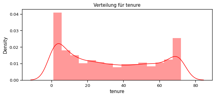
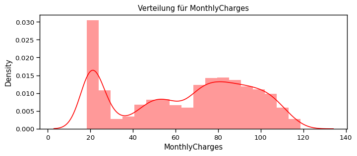
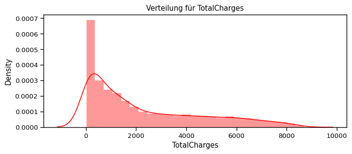
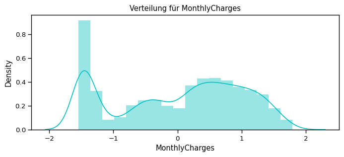
[70]:
def distplot(feature, frame, color="r"):
    plt.figure(figsize=(8,3))
    plt.title("Verteilung für {}".format(feature))
    ax = sns.distplot(frame[feature], color= color)

num_cols = ["tenure", "MonthlyCharges", "TotalCharges"]
for feat in num_cols: distplot(feat, df)
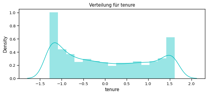
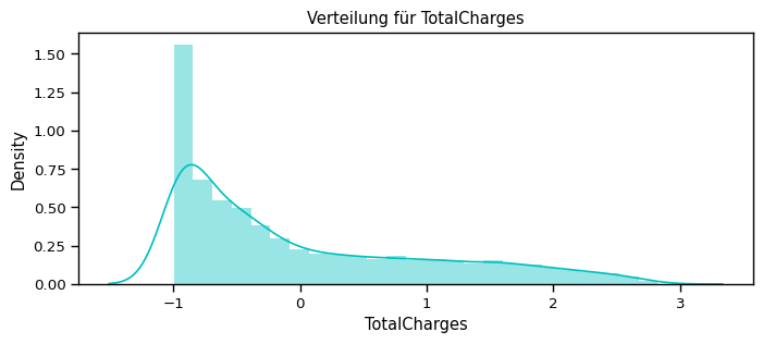
Überlegung: Welchen Scaler sollte ich nutzen?
Da die numerischen Features über verschiedene Wertebereiche (value ranges) verteilt sind, können wir hier den Standard Scalar nutzen, um sie alle auf den gleichen Bereich runterzuskalieren.
Normalisiere die numerischen Attribute
[71]:
df_std = pd.DataFrame(StandardScaler().fit_transform(df[num_cols].astype('float64')),
                       columns=num_cols)
for feat in numerical_cols: distplot(feat, df_std, color='c')
…
[72]:
scaler= StandardScaler()

X_train[num_cols] = scaler.fit_transform(X_train[num_cols])
X_test[num_cols] = scaler.transform(X_test[num_cols])
Modellieren
Es handelt sich hierbei um einen Datensatz mit klar definierten Labels (Churn: Yes oder No), die eine Klassifikationsproblematik beschreiben.
Dazu werden wir nun mehrere Klassifikationsmodelle testen.
K-Nearest Neighbor Classifier
Der K-Nearest-Neighbor Classifier ist eine nichtparametrische Methode zur Schätzung von Wahrscheinlichkeitsdichtefunktionen, mehr Details: https://de.wikipedia.org/wiki/N%C3%A4chste-Nachbarn-Klassifikation
Hier nutzen wir die kNN-Implemtation von scikit-learn: https://scikit-learn.org/stable/modules/generated/sklearn.neighbors.KNeighborsClassifier.html
[73]:
# Initiere das knn-Modell

knn_model = KNeighborsClassifier(n_neighbors = 11)
[74]:
# Trainiere das Modell mit unseren Trainingsdaten

knn_model.fit(X_train,y_train)
[74]:
KNeighborsClassifier(n_neighbors=11)In a Jupyter environment, please rerun this cell to show the HTML representation or trust the notebook.
On GitHub, the HTML representation is unable to render, please try loading this page with nbviewer.org.
Parameters
[75]:
# die "score"-Funktion scoret direkt die predicted Resultate vom X_test gegen die wahren y-Werte und gibt die Accuracy zurück

accuracy_knn = knn_model.score(X_test,y_test)
print("KNN accuracy:",accuracy_knn)
print(knn_model.score(X_test,y_test))
KNN accuracy: 0.7611374407582938
0.7611374407582938
[76]:
# Alternativ kann man direkt mit dem Modell auf den X_test (Testdatensatz) vorhersagen und diese Vorhersagen gegen die wahren Werte des Testdatensatzes mit sklearn evaluieren

y_pred = knn_model.predict(X_test)
prec = precision_score(y_test, y_pred, average=None)
recall = recall_score(y_test, y_pred, average=None)
print("precision: ", prec)
print("recall: ", recall)
precision:  [0.81119714 0.56612529]
recall:  [0.87927695 0.43493761]
[77]:
# Zudem gibt es den "Classification Report", der direkt mehrere Metriken Resultate ausgibt

print(classification_report(y_test, y_pred))
              precision    recall  f1-score   support

           0       0.81      0.88      0.84      1549
           1       0.57      0.43      0.49       561

    accuracy                           0.76      2110
   macro avg       0.69      0.66      0.67      2110
weighted avg       0.75      0.76      0.75      2110
[78]:
# Predict directly with the trained model

y_pred = knn_model.predict(X_test)
print(y_pred)
[0 1 0 ... 0 0 0]
Logistic Regression Classifier
Der Logistic Regression Classifier basiert auf Linear Regression, nur gibt sie am Ende eine
[79]:
lr_model = LogisticRegression()
lr_model.fit(X_train,y_train)
accuracy_lr = lr_model.score(X_test,y_test)
print("Logistic Regression accuracy is :",accuracy_lr)
Logistic Regression accuracy is : 0.776303317535545
[80]:
# Make predictions
lr_pred= lr_model.predict(X_test)
report = classification_report(y_test,lr_pred)
print(report)
              precision    recall  f1-score   support

           0       0.81      0.90      0.86      1549
           1       0.61      0.42      0.50       561

    accuracy                           0.78      2110
   macro avg       0.71      0.66      0.68      2110
weighted avg       0.76      0.78      0.76      2110
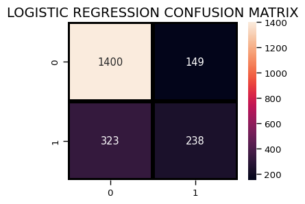
[81]:
plt.figure(figsize=(4,3))
sns.heatmap(confusion_matrix(y_test, lr_pred),
                annot=True,fmt = "d",linecolor="k",linewidths=3)

plt.title("LOGISTIC REGRESSION CONFUSION MATRIX",fontsize=14)
plt.show()
Decision Tree Classifier
[82]:
dt_model = DecisionTreeClassifier()
dt_model.fit(X_train,y_train)
predictdt_y = dt_model.predict(X_test)
accuracy_dt = dt_model.score(X_test,y_test)
print("Decision Tree accuracy is :",accuracy_dt)
Decision Tree accuracy is : 0.7018957345971564
[83]:
print(classification_report(y_test, predictdt_y))
              precision    recall  f1-score   support

           0       0.80      0.79      0.80      1549
           1       0.44      0.45      0.45       561

    accuracy                           0.70      2110
   macro avg       0.62      0.62      0.62      2110
weighted avg       0.70      0.70      0.70      2110
AdaBoost Classifier
[84]:
a_model = AdaBoostClassifier()
a_model.fit(X_train,y_train)
a_preds = a_model.predict(X_test)
print("AdaBoost Classifier accuracy")
metrics.accuracy_score(y_test, a_preds)
AdaBoost Classifier accuracy
[84]:
0.7838862559241706
[85]:
print(classification_report(y_test, a_preds))
              precision    recall  f1-score   support

           0       0.82      0.90      0.86      1549
           1       0.63      0.47      0.53       561

    accuracy                           0.78      2110
   macro avg       0.72      0.68      0.70      2110
weighted avg       0.77      0.78      0.77      2110
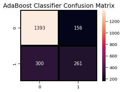
[86]:
plt.figure(figsize=(4,3))
sns.heatmap(confusion_matrix(y_test, a_preds),
                annot=True,fmt = "d",linecolor="k",linewidths=3)

plt.title("AdaBoost Classifier Confusion Matrix",fontsize=14)
plt.show()
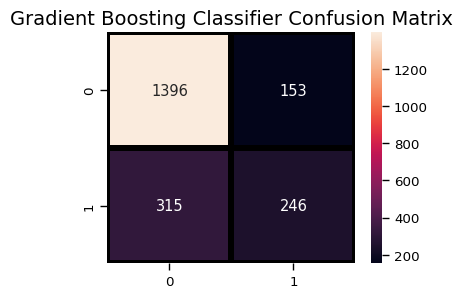
Gradient Boosting Classifier
[87]:
gb = GradientBoostingClassifier()
gb.fit(X_train, y_train)
gb_pred = gb.predict(X_test)
print("Gradient Boosting Classifier", accuracy_score(y_test, gb_pred))
Gradient Boosting Classifier 0.7781990521327015
[88]:
print(classification_report(y_test, gb_pred))
              precision    recall  f1-score   support

           0       0.82      0.90      0.86      1549
           1       0.62      0.44      0.51       561

    accuracy                           0.78      2110
   macro avg       0.72      0.67      0.68      2110
weighted avg       0.76      0.78      0.76      2110
[89]:
plt.figure(figsize=(4,3))
sns.heatmap(confusion_matrix(y_test, gb_pred),
                annot=True,fmt = "d",linecolor="k",linewidths=3)

plt.title("Gradient Boosting Classifier Confusion Matrix",fontsize=14)
plt.show()
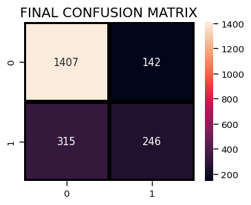
Voting Classifier
Der Voting Classifier ist ein Mixture Modell, der mehrere Modelle vereint, die alle ihre Predictions machen und dann über Majority voting entschieden wird, welche Prediction Output rausgegeben wird.
[90]:
from sklearn.ensemble import VotingClassifier
clf1 = GradientBoostingClassifier()
clf2 = LogisticRegression()
clf3 = AdaBoostClassifier()
eclf1 = VotingClassifier(estimators=[("gbc", clf1), ("lr", clf2), ("abc", clf3)], voting="soft")
eclf1.fit(X_train, y_train)
predictions = eclf1.predict(X_test)
print("Final Accuracy Score ")
print(accuracy_score(y_test, predictions))
Final Accuracy Score
0.7834123222748816
[91]:
print(classification_report(y_test, predictions))
              precision    recall  f1-score   support

           0       0.82      0.91      0.86      1549
           1       0.63      0.44      0.52       561

    accuracy                           0.78      2110
   macro avg       0.73      0.67      0.69      2110
weighted avg       0.77      0.78      0.77      2110
[92]:
plt.figure(figsize=(4,3))
sns.heatmap(confusion_matrix(y_test, predictions),
                annot=True,fmt = "d",linecolor="k",linewidths=3)

plt.title("FINAL CONFUSION MATRIX",fontsize=14)
plt.show()