ML Data Construction Showcase

Revenue Forecasting From Multi-Source Data (Synthetic E-commerce Example)

Learning objectives

• Build a realistic ML-ready dataset from master data + event logs.

• Construct a target label from business logic: future 90-day revenue.

• Engineer behavioral features from historical transactions.

• Encode categorical variables with one-hot encoding.

• Prevent temporal leakage via strict observation vs prediction windows.

Business framing

For each customer at reference date t, predict revenue in the next 90 days. This mirrors production ML settings where we only have historical data at prediction time, while labels come from future outcomes.

import numpy as np
import pandas as pd
from datetime import timedelta

from sklearn.compose import ColumnTransformer
from sklearn.preprocessing import OneHotEncoder

# Set the random seed for reproducibility
SEED = 42
# Create a random number generator with the specified seed
rng = np.random.default_rng(SEED)
np.random.seed(SEED)
print(f"Random seed set to {SEED}")

Random seed set to 42

SECTION B — Generate Synthetic Raw Data

SECTION B.1 — Generate Synthetic Customer Master Table

# Synthetic customer master table
n_customers = 1200

# Define the range of customer IDs
customer_ids = [f"C{i:04d}" for i in range(1, n_customers + 1)]

# Define the values for the categorical features
countries = ["DE", "FR", "CH", "IT", "ES"]
segments = ["Budget", "Standard", "Premium"]
channels = ["Organic", "Paid Ads", "Referral", "Affiliate"]

# Use a fixed synthetic timeline so notebook behavior is deterministic
synthetic_today = pd.Timestamp("2025-01-31")
signup_start = synthetic_today - pd.Timedelta(days=730)  # last 24 months
# Generate random signup dates for each customer
signup_offsets = rng.integers(0, 731, size=n_customers)
signup_dates = signup_start + pd.to_timedelta(signup_offsets, unit="D")

# Create a DataFrame with the generated data
customers = pd.DataFrame(
    {
        "customer_id": customer_ids,
        "signup_date": pd.to_datetime(signup_dates),
        "country": rng.choice(countries, size=n_customers, p=[0.25, 0.2, 0.15, 0.2, 0.2]),
        "customer_segment": rng.choice(segments, size=n_customers, p=[0.4, 0.45, 0.15]),
        "acquisition_channel": rng.choice(channels, size=n_customers, p=[0.35, 0.3, 0.2, 0.15]),
    }
)

customers.head()

	customer_id	signup_date	country	customer_segment	acquisition_channel
0	C0001	2023-04-07	CH	Standard	Referral
1	C0002	2024-08-19	IT	Standard	Paid Ads
2	C0003	2024-05-24	ES	Budget	Organic
3	C0004	2023-12-18	IT	Standard	Referral
4	C0005	2023-12-14	ES	Standard	Organic

Section B.2. Generate synthetic transaction event table

# Synthetic transaction event table
# Design choices as underlying assumptions & distributional choices:
# - Premium customers spend more
# - Paid Ads customers tend to churn more / have fewer repeat purchases
# - Some customers have no transactions
# - Mild recency + seasonality effects

transaction_rows = []

# Define the range of transaction dates
tx_global_start = synthetic_today - pd.Timedelta(days=420)  # >12 months history
tx_global_end = synthetic_today + pd.Timedelta(days=120)    # includes future wrt reference date

# Define the multipliers for the segment frequency and amount
segment_freq_mult = {"Budget": 0.8, "Standard": 1.0, "Premium": 1.35}
segment_amount_mult = {"Budget": 0.75, "Standard": 1.0, "Premium": 1.8}
channel_freq_mult = {"Organic": 1.1, "Paid Ads": 0.75, "Referral": 1.05, "Affiliate": 0.9}
channel_no_tx_bonus = {"Organic": 0.00, "Paid Ads": 0.12, "Referral": 0.00, "Affiliate": 0.03}

# Iterate over each customer in the customers DataFrame
for row in customers.itertuples(index=False):
    cid = row.customer_id
    signup = row.signup_date
    seg = row.customer_segment
    ch = row.acquisition_channel

    # Customers with short tenure have fewer possible transactions
    tenure_days = max((synthetic_today - signup).days, 1)
    tenure_factor = min(tenure_days / 365.0, 1.4)

    # Calculate the base lambda for the Poisson distribution
    base_lambda = 4.5 * segment_freq_mult[seg] * channel_freq_mult[ch] * tenure_factor

    # Probability of no transactions at all
    p_no_tx = 0.08 + channel_no_tx_bonus[ch]
    if rng.random() < p_no_tx:
        continue

    # Generate the number of transactions for the customer following a Poisson distribution with the base lambda
    n_tx = rng.poisson(base_lambda)
    if n_tx <= 0:
        n_tx = 1

    # Mild recency effect: some users get extra recent transactions
    if rng.random() < 0.25:
        n_tx += rng.integers(1, 4)

    # Define the range of transaction dates
    tx_start = max(tx_global_start, signup)
    tx_end = tx_global_end
    n_days = max((tx_end - tx_start).days, 1)

    # Build date weights: slightly more recent + mild seasonal bump in Nov/Dec
    date_index = pd.date_range(tx_start, tx_end, freq="D")
    recency_weight = np.linspace(0.8, 1.2, len(date_index))
    seasonal_weight = np.where(date_index.month.isin([11, 12]), 1.15, 1.0)
    day_weights = recency_weight * seasonal_weight
    day_weights = day_weights / day_weights.sum()

    # Choose the transaction dates for the customer from the date_index array
    chosen_dates = rng.choice(date_index, size=n_tx, replace=True, p=day_weights)

    # Iterate over the chosen transaction dates
    for tx_date in chosen_dates:
        # Log-normal amount with segment effect + occasional outliers
        amount = rng.lognormal(mean=3.6, sigma=0.55) * segment_amount_mult[seg]

        # Occasionally generate outlier purchases
        if rng.random() < 0.015:
            amount *= rng.uniform(5, 12)  # outlier purchases

        # Small seasonal uplift around Nov/Dec
        if pd.Timestamp(tx_date).month in [11, 12]:
            amount *= 1.08

        # Append the transaction data to the transaction_rows list
        transaction_rows.append(
            {
                "customer_id": cid,
                "transaction_date": pd.Timestamp(tx_date),
                "amount": float(round(amount, 2)),
            }
        )

# Convert the transaction_rows list into a DataFrame
transactions = pd.DataFrame(transaction_rows)
# Sort the transactions by customer ID and transaction date
transactions = transactions.sort_values(["customer_id", "transaction_date"]).reset_index(drop=True)
# Display the first few rows of the transactions DataFrame
transactions.head()

	customer_id	transaction_date	amount
0	C0001	2024-02-18	30.96
1	C0001	2024-04-14	24.45
2	C0001	2024-07-15	44.53
3	C0001	2024-09-05	34.86
4	C0001	2024-11-07	23.09

# Basic sanity checks
print("Customers head:")
display(customers.head())

# Display the first few rows of the transactions DataFrame
print("\nTransactions head:")
display(transactions.head())

# Print the row counts for the customers and transactions DataFrames
print("\nRow counts")
print("customers:", len(customers))
print("transactions:", len(transactions))

# Print the number of unique customers in the customers and transactions DataFrames
print("\nUnique customers")
print("customers table:", customers["customer_id"].nunique())
print("transactions table:", transactions["customer_id"].nunique())

# Calculate the number of customers with no transactions
customers_with_no_tx = customers.loc[~customers["customer_id"].isin(transactions["customer_id"]), "customer_id"].nunique()
print("customers with no transactions:", customers_with_no_tx)

# Print the number of missing values in the customers and transactions DataFrames
print("\nMissing values")
print("customers:\n", customers.isna().sum())
print("transactions:\n", transactions.isna().sum())

Customers head:

	customer_id	signup_date	country	customer_segment	acquisition_channel
0	C0001	2023-04-07	CH	Standard	Referral
1	C0002	2024-08-19	IT	Standard	Paid Ads
2	C0003	2024-05-24	ES	Budget	Organic
3	C0004	2023-12-18	IT	Standard	Referral
4	C0005	2023-12-14	ES	Standard	Organic

Transactions head:

	customer_id	transaction_date	amount
0	C0001	2024-02-18	30.96
1	C0001	2024-04-14	24.45
2	C0001	2024-07-15	44.53
3	C0001	2024-09-05	34.86
4	C0001	2024-11-07	23.09

Row counts
customers: 1200
transactions: 4636

Unique customers
customers table: 1200
transactions table: 1046
customers with no transactions: 154

Missing values
customers:
 customer_id            0
signup_date            0
country                0
customer_segment       0
acquisition_channel    0
dtype: int64
transactions:
 customer_id         0
transaction_date    0
amount              0
dtype: int64

# Save the synthetic data to a CSV file
customers.to_csv("data/customers.csv", index=False)
transactions.to_csv("data/transactions.csv", index=False)


print("Synthetic data saved to CSV files")

Synthetic data saved to CSV files

SECTION C — Define Temporal Windows and Reference Date

Now, we have (synthesized) our raw data set. Often this is the starting point of data that you get from your business stakeholders.

Next, we must separate:

• Observation window: historical data used to build features.

• Prediction window: future period used to construct the label.

If we accidentally include prediction-window information in features, we create temporal leakage.

# Reference date and windows
# Choose t so we still have enough future transactions to build labels
reference_date = transactions["transaction_date"].max() - pd.Timedelta(days=120)

# Define the observation and prediction windows in days, as discussed in the slides
observation_days = 180
prediction_days = 90

# Calculate the start and end dates for the observation and prediction windows
obs_start = reference_date - pd.Timedelta(days=observation_days)
obs_end = reference_date

# Calculate the start and end dates for the prediction window
pred_start = reference_date
pred_end = reference_date + pd.Timedelta(days=prediction_days)

# Print the reference date and the observation and prediction windows
print("reference_date (t):", reference_date.date())
print(f"observation window: [{obs_start.date()}, {obs_end.date()}]")
print(f"prediction window: ({pred_start.date()}, {pred_end.date()}]")

reference_date (t): 2025-01-31
observation window: [2024-08-04, 2025-01-31]
prediction window: (2025-01-31, 2025-05-01]

SECTION D — Label Construction (Future Revenue)

Define target for customer i as:

[ y_i = \sum `:nbsphinx-math:text{amount}`_{i, d} \text{ for } d :nbsphinx-math:`in `(t, t+90] ]

Customers with no transactions in the prediction window get label 0.

# Prediction-window transactions: (t, t+90]
pred_tx = transactions[
    (transactions["transaction_date"] > pred_start)
    & (transactions["transaction_date"] <= pred_end)
].copy()

# Group the transactions by customer ID and sum the amount for each customer
label_df = (
    pred_tx.groupby("customer_id", as_index=False)["amount"]
    .sum()
    .rename(columns={"amount": "future_revenue_90d"})
)

# Ensure every customer exists in label table
label_df = customers[["customer_id"]].merge(label_df, on="customer_id", how="left")
label_df["future_revenue_90d"] = label_df["future_revenue_90d"].fillna(0.0)

# Print a summary of the label distribution
print("Label summary:")
print(label_df["future_revenue_90d"].describe())

# Calculate the percentage of zero labels
pct_zero = (label_df["future_revenue_90d"] == 0).mean() * 100
print(f"Percent zero labels: {pct_zero:.2f}%")

Label summary:
count    1200.000000
mean       46.428433
std        80.516101
min         0.000000
25%         0.000000
50%        19.955000
75%        62.417500
max      1070.010000
Name: future_revenue_90d, dtype: float64
Percent zero labels: 45.17%

SECTION E — Feature Engineering From Observation Window (Past Behavior)

We engineer RFM-style and trend features only from historical data in [t-180, t].

No transaction after t is used for features (prevents leakage).

SECTION E.1: Define the range of the past 180 days

# Observation-window transactions: [t-180, t], i.e. 180 days before t
obs_tx = transactions[
    (transactions["transaction_date"] >= obs_start)
    & (transactions["transaction_date"] <= obs_end)
].copy()
obs_tx["tx_day"] = obs_tx["transaction_date"].dt.normalize()

obs_tx.head()

	customer_id	transaction_date	amount	tx_day
3	C0001	2024-09-05	34.86	2024-09-05
4	C0001	2024-11-07	23.09	2024-11-07
5	C0001	2025-01-06	54.76	2025-01-06
13	C0004	2024-09-20	27.63	2024-09-20
14	C0004	2024-10-24	20.84	2024-10-24

SECTION E.2. Core Behavior Features

# Core behavior features in observation window
# Group by customer ID and calculate the following metrics:
# - last_purchase_date: the latest transaction date for each customer
# - frequency: the number of transactions for each customer
# - monetary_total: the total amount spent by each customer
# - active_days: the number of unique days on which each customer has made a purchase
obs_agg = obs_tx.groupby("customer_id").agg(
    last_purchase_date=("transaction_date", "max"),
    frequency=("amount", "count"),
    monetary_total=("amount", "sum"),
    active_days=("tx_day", "nunique"),
)
# Calculate the average order value for each customer
obs_agg["avg_order_value"] = obs_agg["monetary_total"] / obs_agg["frequency"]
obs_agg = obs_agg.reset_index()

# Recency (days since last purchase)
obs_agg["recency_days"] = (reference_date - obs_agg["last_purchase_date"]).dt.days

obs_agg.head()

	customer_id	last_purchase_date	frequency	monetary_total	active_days	avg_order_value	recency_days
0	C0001	2025-01-06	3	112.71	3	37.570	25
1	C0004	2024-10-24	2	48.47	2	24.235	99
2	C0005	2024-12-01	1	49.24	1	49.240	61
3	C0008	2024-12-16	2	80.94	2	40.470	46
4	C0009	2024-12-01	2	171.99	2	85.995	61

SECTION E.3. Trend features

# Calculate the sum of the amount for each customer in the recent 30 days
recent_30d = obs_tx[
    (obs_tx["transaction_date"] > (reference_date - pd.Timedelta(days=30)))
    & (obs_tx["transaction_date"] <= reference_date)
]

# Calculate the sum of the amount for each customer in the previous 30 days
prev_30d = obs_tx[
    (obs_tx["transaction_date"] > (reference_date - pd.Timedelta(days=60)))
    & (obs_tx["transaction_date"] <= (reference_date - pd.Timedelta(days=30)))
]

# Calculate the sum of the amount for each customer in the recent 30 days
recent_30d_spend = (
    recent_30d.groupby("customer_id", as_index=False)["amount"]
    .sum()
    .rename(columns={"amount": "recent_30d_spend"})
)

# Calculate the sum of the amount for each customer in the previous 30 days
prev_30d_spend = (
    prev_30d.groupby("customer_id", as_index=False)["amount"]
    .sum()
    .rename(columns={"amount": "prev_30d_spend"})
)

# Merge the recent 30 days spend and previous 30 days spend into the observation aggregate DataFrame
features_df = obs_agg.merge(recent_30d_spend, on="customer_id", how="left")
features_df = features_df.merge(prev_30d_spend, on="customer_id", how="left")
features_df[["recent_30d_spend", "prev_30d_spend"]] = features_df[["recent_30d_spend", "prev_30d_spend"]].fillna(0.0)
features_df["spend_trend"] = features_df["recent_30d_spend"] - features_df["prev_30d_spend"]

features_df.head()

	customer_id	last_purchase_date	frequency	monetary_total	active_days	avg_order_value	recency_days	recent_30d_spend	prev_30d_spend	spend_trend
0	C0001	2025-01-06	3	112.71	3	37.570	25	54.76	0.00	54.76
1	C0004	2024-10-24	2	48.47	2	24.235	99	0.00	0.00	0.00
2	C0005	2024-12-01	1	49.24	1	49.240	61	0.00	0.00	0.00
3	C0008	2024-12-16	2	80.94	2	40.470	46	0.00	34.31	-34.31
4	C0009	2024-12-01	2	171.99	2	85.995	61	0.00	0.00	0.00

Data Cleansing!!

Missing-value handling choices:

• Customers with no observation-window transactions get frequency=0, monetary_total=0, active_days=0, recent_30d_spend=0, prev_30d_spend=0, spend_trend=0.

• avg_order_value is set to 0 when frequency=0.

• recency_days is set to a large value (observation_days + 1) for „not recently active“ customers.

# Merge engineered features into customer table
model_base = customers.merge(features_df, on="customer_id", how="left")

# Fill missing values with 0.0 for the following columns
fill_zero_cols = [
    "frequency",
    "monetary_total",
    "active_days",
    "recent_30d_spend",
    "prev_30d_spend",
    "spend_trend",
]

# Fill missing values with 0.0 for the following columns
for col in fill_zero_cols:
    model_base[col] = model_base[col].fillna(0.0)

# Fill missing values with a large value for the following columns
model_base["recency_days"] = model_base["recency_days"].fillna(observation_days + 1)
model_base["avg_order_value"] = model_base["avg_order_value"].fillna(0.0)

# last_purchase_date is not used as model feature directly
model_base = model_base.drop(columns=["last_purchase_date"], errors="ignore")

model_base.head()

	customer_id	signup_date	country	customer_segment	acquisition_channel	frequency	monetary_total	active_days	avg_order_value	recency_days	recent_30d_spend	prev_30d_spend	spend_trend
0	C0001	2023-04-07	CH	Standard	Referral	3.0	112.71	3.0	37.570	25.0	54.76	0.0	54.76
1	C0002	2024-08-19	IT	Standard	Paid Ads	0.0	0.00	0.0	0.000	181.0	0.00	0.0	0.00
2	C0003	2024-05-24	ES	Budget	Organic	0.0	0.00	0.0	0.000	181.0	0.00	0.0	0.00
3	C0004	2023-12-18	IT	Standard	Referral	2.0	48.47	2.0	24.235	99.0	0.00	0.0	0.00
4	C0005	2023-12-14	ES	Standard	Organic	1.0	49.24	1.0	49.240	61.0	0.00	0.0	0.00

SECTION F — Add Tenure Feature

model_base["tenure_days"] = (reference_date - model_base["signup_date"]).dt.days
model_base[["customer_id", "signup_date", "tenure_days"]].head()

model_base.head()

	customer_id	signup_date	country	customer_segment	acquisition_channel	frequency	monetary_total	active_days	avg_order_value	recency_days	recent_30d_spend	prev_30d_spend	spend_trend	tenure_days
0	C0001	2023-04-07	CH	Standard	Referral	3.0	112.71	3.0	37.570	25.0	54.76	0.0	54.76	665
1	C0002	2024-08-19	IT	Standard	Paid Ads	0.0	0.00	0.0	0.000	181.0	0.00	0.0	0.00	165
2	C0003	2024-05-24	ES	Budget	Organic	0.0	0.00	0.0	0.000	181.0	0.00	0.0	0.00	252
3	C0004	2023-12-18	IT	Standard	Referral	2.0	48.47	2.0	24.235	99.0	0.00	0.0	0.00	410
4	C0005	2023-12-14	ES	Standard	Organic	1.0	49.24	1.0	49.240	61.0	0.00	0.0	0.00	414

SECTION G — Handle Categorical Features (One-Hot Encoding)

Categorical fields (country, customer_segment, acquisition_channel) cannot be used directly by most ML models. We one-hot encode them into binary indicator columns.

We avoid arbitrary ordinal encoding here because there is no meaningful numeric order between categories.

# Identify the column types so far
model_base.dtypes

customer_id                       str
signup_date            datetime64[us]
country                           str
customer_segment                  str
acquisition_channel               str
frequency                     float64
monetary_total                float64
active_days                   float64
avg_order_value               float64
recency_days                  float64
recent_30d_spend              float64
prev_30d_spend                float64
spend_trend                   float64
tenure_days                     int64
dtype: object

# Select the categorical columns dedicatedly
categorical_cols = ["country", "customer_segment", "acquisition_channel"]
numeric_cols = [
    "recency_days",
    "frequency",
    "monetary_total",
    "avg_order_value",
    "active_days",
    "recent_30d_spend",
    "prev_30d_spend",
    "spend_trend",
    "tenure_days",
]

# Keep a clean feature frame (exclude identifiers/date columns)
feature_input = model_base[["customer_id", "signup_date"] + categorical_cols + numeric_cols].copy()

feature_input.head()

	customer_id	signup_date	country	customer_segment	acquisition_channel	recency_days	frequency	monetary_total	avg_order_value	active_days	recent_30d_spend	prev_30d_spend	spend_trend	tenure_days
0	C0001	2023-04-07	CH	Standard	Referral	25.0	3.0	112.71	37.570	3.0	54.76	0.0	54.76	665
1	C0002	2024-08-19	IT	Standard	Paid Ads	181.0	0.0	0.00	0.000	0.0	0.00	0.0	0.00	165
2	C0003	2024-05-24	ES	Budget	Organic	181.0	0.0	0.00	0.000	0.0	0.00	0.0	0.00	252
3	C0004	2023-12-18	IT	Standard	Referral	99.0	2.0	48.47	24.235	2.0	0.00	0.0	0.00	410
4	C0005	2023-12-14	ES	Standard	Organic	61.0	1.0	49.24	49.240	1.0	0.00	0.0	0.00	414

# One-hot encode the categorical columns
preprocessor = ColumnTransformer(
    transformers=[
        ("cat", OneHotEncoder(handle_unknown="ignore", sparse_output=False), categorical_cols),
        ("num", "passthrough", numeric_cols),
    ]
)

# Fit the preprocessor on the feature input
X_array = preprocessor.fit_transform(feature_input[categorical_cols + numeric_cols])

# Get the feature names from the preprocessor
cat_feature_names = preprocessor.named_transformers_["cat"].get_feature_names_out(categorical_cols).tolist()
final_feature_names = cat_feature_names + numeric_cols

# Create a DataFrame with the one-hot encoded features
X = pd.DataFrame(X_array, columns=final_feature_names, index=feature_input.index)

# Print the number of one-hot columns created and the total number of feature columns in X
print("One-hot columns created:", len(cat_feature_names))
print("Total feature columns in X:", X.shape[1])
X.head()

One-hot columns created: 12
Total feature columns in X: 21

	country_CH	country_DE	country_ES	country_FR	country_IT	customer_segment_Budget	customer_segment_Premium	customer_segment_Standard	acquisition_channel_Affiliate	acquisition_channel_Organic	...	acquisition_channel_Referral	recency_days	frequency	monetary_total	avg_order_value	active_days	recent_30d_spend	prev_30d_spend	spend_trend	tenure_days
0	1.0	0.0	0.0	0.0	0.0	0.0	0.0	1.0	0.0	0.0	...	1.0	25.0	3.0	112.71	37.570	3.0	54.76	0.0	54.76	665.0
1	0.0	0.0	0.0	0.0	1.0	0.0	0.0	1.0	0.0	0.0	...	0.0	181.0	0.0	0.00	0.000	0.0	0.00	0.0	0.00	165.0
2	0.0	0.0	1.0	0.0	0.0	1.0	0.0	0.0	0.0	1.0	...	0.0	181.0	0.0	0.00	0.000	0.0	0.00	0.0	0.00	252.0
3	0.0	0.0	0.0	0.0	1.0	0.0	0.0	1.0	0.0	0.0	...	1.0	99.0	2.0	48.47	24.235	2.0	0.00	0.0	0.00	410.0
4	0.0	0.0	1.0	0.0	0.0	0.0	0.0	1.0	0.0	1.0	...	0.0	61.0	1.0	49.24	49.240	1.0	0.00	0.0	0.00	414.0

5 rows × 21 columns

SECTION H — Final Dataset Assembly

# Join target y
final_dataset = pd.concat(
    [
        model_base[["customer_id"]].reset_index(drop=True),
        X.reset_index(drop=True),
        label_df[["future_revenue_90d"]].reset_index(drop=True),
    ],
    axis=1,
)

final_dataset.head()

	customer_id	country_CH	country_DE	country_ES	country_FR	country_IT	customer_segment_Budget	customer_segment_Premium	customer_segment_Standard	acquisition_channel_Affiliate	...	recency_days	frequency	monetary_total	avg_order_value	active_days	recent_30d_spend	prev_30d_spend	spend_trend	tenure_days	future_revenue_90d
0	C0001	1.0	0.0	0.0	0.0	0.0	0.0	0.0	1.0	0.0	...	25.0	3.0	112.71	37.570	3.0	54.76	0.0	54.76	665.0	0.00
1	C0002	0.0	0.0	0.0	0.0	1.0	0.0	0.0	1.0	0.0	...	181.0	0.0	0.00	0.000	0.0	0.00	0.0	0.00	165.0	0.00
2	C0003	0.0	0.0	1.0	0.0	0.0	1.0	0.0	0.0	0.0	...	181.0	0.0	0.00	0.000	0.0	0.00	0.0	0.00	252.0	32.47
3	C0004	0.0	0.0	0.0	0.0	1.0	0.0	0.0	1.0	0.0	...	99.0	2.0	48.47	24.235	2.0	0.00	0.0	0.00	410.0	48.28
4	C0005	0.0	0.0	1.0	0.0	0.0	0.0	0.0	1.0	0.0	...	61.0	1.0	49.24	49.240	1.0	0.00	0.0	0.00	414.0	63.55

5 rows × 23 columns

print("Final dataset shape:", final_dataset.shape)
print("\nSample rows:")
display(final_dataset.head(5))

print("\nLeakage check (date ranges used):")
print(f"Observation window used for features: [{obs_start.date()}, {obs_end.date()}]")
print(f"Prediction window used for label: ({pred_start.date()}, {pred_end.date()}]")
print("No transactions after t are used in feature engineering.")

Final dataset shape: (1200, 23)

Sample rows:

	customer_id	country_CH	country_DE	country_ES	country_FR	country_IT	customer_segment_Budget	customer_segment_Premium	customer_segment_Standard	acquisition_channel_Affiliate	...	recency_days	frequency	monetary_total	avg_order_value	active_days	recent_30d_spend	prev_30d_spend	spend_trend	tenure_days	future_revenue_90d
0	C0001	1.0	0.0	0.0	0.0	0.0	0.0	0.0	1.0	0.0	...	25.0	3.0	112.71	37.570	3.0	54.76	0.0	54.76	665.0	0.00
1	C0002	0.0	0.0	0.0	0.0	1.0	0.0	0.0	1.0	0.0	...	181.0	0.0	0.00	0.000	0.0	0.00	0.0	0.00	165.0	0.00
2	C0003	0.0	0.0	1.0	0.0	0.0	1.0	0.0	0.0	0.0	...	181.0	0.0	0.00	0.000	0.0	0.00	0.0	0.00	252.0	32.47
3	C0004	0.0	0.0	0.0	0.0	1.0	0.0	0.0	1.0	0.0	...	99.0	2.0	48.47	24.235	2.0	0.00	0.0	0.00	410.0	48.28
4	C0005	0.0	0.0	1.0	0.0	0.0	0.0	0.0	1.0	0.0	...	61.0	1.0	49.24	49.240	1.0	0.00	0.0	0.00	414.0	63.55

5 rows × 23 columns

Leakage check (date ranges used):
Observation window used for features: [2024-08-04, 2025-01-31]
Prediction window used for label: (2025-01-31, 2025-05-01]
No transactions after t are used in feature engineering.

SECTION H2 — Pre-ML: Correlation, Redundancy, Scaling & Split

Before feeding the dataset to an ML model, we perform:

1. Pre-ML checks: missing values, duplicates, constant/near-constant columns in the final feature matrix.

2. Correlation analysis: heatmap and identification of highly correlated numeric features (and one-hot redundancy).

3. Redundancy handling: optionally drop one level per categorical (to avoid perfect multicollinearity) and drop numeric pairs above a correlation threshold.

4. Train/validation split: reproducible split for model development (for multiple reference dates in production, use a temporal split).

5. Scaling: fit scaler on training data only, then transform both train and validation to avoid leakage.

# ---------------------------------------------------------------------------
# Pre-ML check: sanity on the final feature matrix (before split/scaling)
# ---------------------------------------------------------------------------

def pre_ml_checks(df, feature_columns, target_column="future_revenue_90d"):
    """
    Run basic sanity checks on the dataset intended for ML.

    Parameters
    ----------
    df : pd.DataFrame
        Full dataset including features and target.
    feature_columns : list of str
        Column names used as features (exclude IDs and target).
    target_column : str
        Name of the target column.

    Returns
    -------
    dict
        Summary of checks: missing, duplicates, constant columns.
    """
    X = df[feature_columns]
    out = {}

    # Missing values
    missing = X.isna().sum()
    out["missing"] = missing[missing > 0]
    if out["missing"].empty:
        out["missing"] = "No missing values in features."

    # Duplicate rows (in feature space)
    out["n_duplicates"] = X.duplicated().sum()

    # Constant or near-constant columns (zero variance)
    constant = []
    for col in X.columns:
        if X[col].nunique() <= 1:
            constant.append(col)
    out["constant_columns"] = constant if constant else "None"

    return out


# Feature columns = everything in final_dataset except ID and target
FEATURE_COLS = [c for c in final_dataset.columns
                if c not in ("customer_id", "future_revenue_90d")]
TARGET_COL = "future_revenue_90d"

checks = pre_ml_checks(final_dataset, FEATURE_COLS, TARGET_COL)

print("Pre-ML checks (final feature matrix):")
print("  Missing per column:", checks["missing"])
print("  Duplicate rows (features):", checks["n_duplicates"])
print("  Constant/near-constant columns:", checks["constant_columns"])

Pre-ML checks (final feature matrix):
  Missing per column: No missing values in features.
  Duplicate rows (features): 2
  Constant/near-constant columns: None

# ---------------------------------------------------------------------------
# Correlation analysis: numeric features only (one-hot dummies are 0/1)
# ---------------------------------------------------------------------------

import matplotlib.pyplot as plt
import seaborn as sns

# Numeric feature columns (same as used in encoding)
NUMERIC_FOR_CORR = [
    "recency_days", "frequency", "monetary_total", "avg_order_value",
    "active_days", "recent_30d_spend", "prev_30d_spend", "spend_trend", "tenure_days",
]

X_numeric = final_dataset[NUMERIC_FOR_CORR]
corr_matrix = X_numeric.corr()

fig, ax = plt.subplots(figsize=(10, 8))
sns.heatmap(corr_matrix, annot=True, fmt=".2f", cmap="RdBu_r", center=0,
            square=True, linewidths=0.5, ax=ax)
ax.set_title("Correlation matrix (numeric features)")
plt.tight_layout()
plt.show()

# Pairs with |correlation| above threshold (e.g. 0.9 or 0.95)
CORR_THRESHOLD = 0.9
high_corr_pairs = []
for i in range(len(corr_matrix.columns)):
    for j in range(i + 1, len(corr_matrix.columns)):
        if abs(corr_matrix.iloc[i, j]) >= CORR_THRESHOLD:
            high_corr_pairs.append(
                (corr_matrix.columns[i], corr_matrix.columns[j], corr_matrix.iloc[i, j])
            )
print(f"\nNumeric pairs with |correlation| >= {CORR_THRESHOLD}:")
if high_corr_pairs:
    for a, b, r in high_corr_pairs:
        print(f"  {a} <-> {b}: {r:.3f}")
else:
    print("  None.")

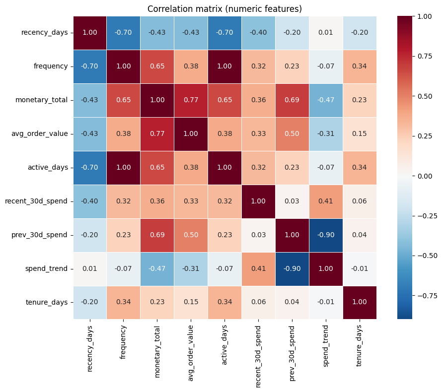
Numeric pairs with |correlation| >= 0.9:
  frequency <-> active_days: 0.998

Interpreting correlation and what to do about it

Which features tend to correlate?

• Numeric behavioural features often move together: e.g. frequency and active_days (both count activity in the observation window), or monetary_total with recent_30d_spend (total spend vs a component of it). avg_order_value is derived as monetary_total / frequency, so it is algebraically tied to those two. In this dataset we may see strong correlations among these.

• One-hot encoded categoricals are perfectly redundant within each group: the columns for one categorical (e.g. all country_*) sum to 1 for every row, so one column is a linear combination of the others.

What can we do?

1. One-hot: Drop one level per categorical (e.g. the first alphabetically). We keep the rest; the dropped level becomes the „reference“ in linear models. This removes perfect multicollinearity within each categorical.

2. Numeric pairs: For pairs with |correlation| above a chosen threshold (e.g. 0.9 or 0.95), we can drop one of the two. Which one to drop is a modelling choice (e.g. keep the one that is easier to interpret or more stable).

Why do it?

• Linear / penalized linear models: High or perfect correlation makes coefficient estimates unstable (large variance) and can break solvers. Dropping redundant columns stabilizes estimates and keeps the model well-defined.

• Interpretability: Fewer redundant features make coefficients easier to interpret (e.g. „effect of country X vs reference“ instead of an ill-defined mix).

• Tree-based models (Random Forest, XGBoost, etc.) are less sensitive to multicollinearity; they can still benefit from fewer noisy/redundant features but do not require this step for numerical stability.

How we implement it below

• For categoricals: we identify one column to drop per group (e.g. first per group) and exclude them from the feature set.

• For numerics: we compute the correlation matrix, find pairs above a threshold (e.g. 0.95), and drop one column from each pair (e.g. the second in a fixed order) so that no remaining pair exceeds the threshold. The next cell implements both steps.

# ---------------------------------------------------------------------------
# Redundancy: one-hot "drop first" and optional removal of highly correlated numerics
# ---------------------------------------------------------------------------

# (1) One-hot encoding created one column per level; for linear models we often
#     drop one level per categorical to avoid perfect multicollinearity.
#     Here we define which columns to drop (one per categorical group).
CATEGORICAL_GROUPS = {
    "country": [c for c in FEATURE_COLS if c.startswith("country_")],
    "customer_segment": [c for c in FEATURE_COLS if c.startswith("customer_segment_")],
    "acquisition_channel": [c for c in FEATURE_COLS if c.startswith("acquisition_channel_")],
}

# Drop the first alphabetically (e.g. country_CH, customer_segment_Budget, acquisition_channel_Affiliate)
COLS_TO_DROP_ONEHOT = [cols[0] for cols in CATEGORICAL_GROUPS.values()]
print("One-hot columns dropped (one per group) to avoid multicollinearity:", COLS_TO_DROP_ONEHOT)

# (2) Optionally drop one of each highly correlated numeric pair (keep first, drop second)
def get_columns_to_drop_high_corr(corr_matrix, threshold=0.95):
    """Return a set of column names to drop so that no pair has |corr| >= threshold."""
    to_drop = set()
    for i in range(len(corr_matrix.columns)):
        for j in range(i + 1, len(corr_matrix.columns)):
            if abs(corr_matrix.iloc[i, j]) >= threshold:
                # Drop the second column (j)
                to_drop.add(corr_matrix.columns[j])
    return to_drop


HIGH_CORR_DROP_THRESHOLD = 0.95
cols_drop_high_corr = get_columns_to_drop_high_corr(corr_matrix, HIGH_CORR_DROP_THRESHOLD)
print(f"\nNumeric columns to drop (|corr| >= {HIGH_CORR_DROP_THRESHOLD}):", cols_drop_high_corr or "None")

# Build the reduced feature list (optional: apply both one-hot drop and high-corr drop)
FEATURE_COLS_REDUCED = [
    c for c in FEATURE_COLS
    if c not in COLS_TO_DROP_ONEHOT and c not in cols_drop_high_corr
]
print(f"\nFeature count: original = {len(FEATURE_COLS)}, reduced = {len(FEATURE_COLS_REDUCED)}")

One-hot columns dropped (one per group) to avoid multicollinearity: ['country_CH', 'customer_segment_Budget', 'acquisition_channel_Affiliate']

Numeric columns to drop (|corr| >= 0.95): {'active_days'}

Feature count: original = 21, reduced = 17

data_final = final_dataset[FEATURE_COLS_REDUCED+[TARGET_COL]]
print(data_final.info())
data_final.head()

<class 'pandas.DataFrame'>
RangeIndex: 1200 entries, 0 to 1199
Data columns (total 18 columns):
 #   Column                        Non-Null Count  Dtype
---  ------                        --------------  -----
 0   country_DE                    1200 non-null   float64
 1   country_ES                    1200 non-null   float64
 2   country_FR                    1200 non-null   float64
 3   country_IT                    1200 non-null   float64
 4   customer_segment_Premium      1200 non-null   float64
 5   customer_segment_Standard     1200 non-null   float64
 6   acquisition_channel_Organic   1200 non-null   float64
 7   acquisition_channel_Paid Ads  1200 non-null   float64
 8   acquisition_channel_Referral  1200 non-null   float64
 9   recency_days                  1200 non-null   float64
 10  frequency                     1200 non-null   float64
 11  monetary_total                1200 non-null   float64
 12  avg_order_value               1200 non-null   float64
 13  recent_30d_spend              1200 non-null   float64
 14  prev_30d_spend                1200 non-null   float64
 15  spend_trend                   1200 non-null   float64
 16  tenure_days                   1200 non-null   float64
 17  future_revenue_90d            1200 non-null   float64
dtypes: float64(18)
memory usage: 168.9 KB
None

	country_DE	country_ES	country_FR	country_IT	customer_segment_Premium	customer_segment_Standard	acquisition_channel_Organic	acquisition_channel_Paid Ads	acquisition_channel_Referral	recency_days	frequency	monetary_total	avg_order_value	recent_30d_spend	prev_30d_spend	spend_trend	tenure_days	future_revenue_90d
0	0.0	0.0	0.0	0.0	0.0	1.0	0.0	0.0	1.0	25.0	3.0	112.71	37.570	54.76	0.0	54.76	665.0	0.00
1	0.0	0.0	0.0	1.0	0.0	1.0	0.0	1.0	0.0	181.0	0.0	0.00	0.000	0.00	0.0	0.00	165.0	0.00
2	0.0	1.0	0.0	0.0	0.0	0.0	1.0	0.0	0.0	181.0	0.0	0.00	0.000	0.00	0.0	0.00	252.0	32.47
3	0.0	0.0	0.0	1.0	0.0	1.0	0.0	0.0	1.0	99.0	2.0	48.47	24.235	0.00	0.0	0.00	410.0	48.28
4	0.0	1.0	0.0	0.0	0.0	1.0	1.0	0.0	0.0	61.0	1.0	49.24	49.240	0.00	0.0	0.00	414.0	63.55

# save the final dataset to a CSV file
data_final.to_csv("data/final_dataset.csv", sep=";", index=False)

We have finished (showcasing) feature engineering, but still need to normalize (as an example of preprocessing steps) the data before we can feed it to train the model.

Why we still need preprocessing

• Many models are sensitive to feature scale (e.g., linear models with regularization, kNN, neural nets). Without scaling, large-magnitude features (e.g. monetary_total, tenure_days) can dominate the objective and distort learning.

• Some preprocessing steps are required for numerical stability and interpretability (e.g., removing perfect multicollinearity from one-hot encoded categoricals).

When to do preprocessing?

Normalization (and similar preprocessing) must be fitted after the train/validation split.

Even though we have saved final_dataset.csv, the data is not yet in the form we should feed directly into many ML algorithms.

Why we split first, then fit preprocessing on train only (leakage avoidance)

Preprocessing often computes statistics from the data (mean/std for scaling, quantiles for clipping, PCA directions, feature selection thresholds, imputation values, etc.). If those statistics are computed using all rows (train + validation), information from the validation set leaks into training.

• Correct pattern:

  1. Split into train/validation.

  2. Fit preprocessing steps using training data only.

  3. Apply (“transform”) the fitted preprocessing to train and validation.

• What goes wrong if we fit preprocessing before the split:

  • The model indirectly “sees” validation distribution information via the preprocessing statistics.

  • Validation metrics become optimistically biased and won’t reflect true generalization.

Note: the correlation-based feature dropping shown above is also a form of feature selection. In a strict pipeline, it should be decided using training data only. For this teaching notebook we compute it once for simplicity, but the same leakage principle applies.

# ---------------------------------------------------------------------------
# Train/validation split (reproducible; for production with multiple reference dates, use temporal split)
# ---------------------------------------------------------------------------

from sklearn.model_selection import train_test_split

SPLIT_SEED = SEED  # use same as notebook
VAL_SIZE = 0.2

# Use reduced feature set if we applied redundancy handling; else use full feature list
X_ml = final_dataset[FEATURE_COLS_REDUCED]
y_ml = final_dataset[TARGET_COL]

X_train, X_val, y_train, y_val = train_test_split(
    X_ml, y_ml, test_size=VAL_SIZE, random_state=SPLIT_SEED, shuffle=True
)

print(f"Train size: {len(X_train)}, Validation size: {len(X_val)}")
print(f"Train target mean: {y_train.mean():.2f}, val target mean: {y_val.mean():.2f}")

Train size: 960, Validation size: 240
Train target mean: 47.12, val target mean: 43.65

As mentioned, after **splitting* into train/validation, we can now

• Fit preprocessing steps using training data only.

• Apply (“transform”) the fitted preprocessing to train and validation.

Separating training and validation data for fitting and applying helps avoid:

• that the model indirectly “sees” validation distribution information via the preprocessing statistics.

• validation metrics become optimistically biased and won’t reflect true generalization.

# ---------------------------------------------------------------------------
# Scaling: fit on training data only, then transform train and validation
# ---------------------------------------------------------------------------

from sklearn.preprocessing import StandardScaler

scaler = StandardScaler()
X_train_scaled = scaler.fit_transform(X_train)
X_val_scaled = scaler.transform(X_val)

# Optional: wrap back into DataFrames for readability
X_train_scaled_df = pd.DataFrame(X_train_scaled, columns=FEATURE_COLS_REDUCED, index=X_train.index)
X_val_scaled_df = pd.DataFrame(X_val_scaled, columns=FEATURE_COLS_REDUCED, index=X_val.index)

print("Scaled feature matrices ready for ML.")
print("X_train_scaled shape:", X_train_scaled.shape)
print("X_val_scaled shape:", X_val_scaled.shape)

Scaled feature matrices ready for ML.
X_train_scaled shape: (960, 17)
X_val_scaled shape: (240, 17)

# ---------------------------------------------------------------------------
# Export train/validation splits (raw + scaled) for downstream modeling
# ---------------------------------------------------------------------------

from pathlib import Path

PROJECT_ROOT = Path.cwd()
PROJECT_ROOT = Path.cwd()
if not (PROJECT_ROOT / "data").is_dir():
    PROJECT_ROOT = PROJECT_ROOT.parent

DATA_DIR = PROJECT_ROOT / "data"
DATA_DIR.mkdir(parents=True, exist_ok=True)

# Raw splits
X_train.to_csv(DATA_DIR / "X_train.csv", index=False)
X_val.to_csv(DATA_DIR / "X_val.csv", index=False)
y_train.to_csv(DATA_DIR / "y_train.csv", index=False, header=[TARGET_COL])
y_val.to_csv(DATA_DIR / "y_val.csv", index=False, header=[TARGET_COL])

# Scaled splits
X_train_scaled_df.to_csv(DATA_DIR / "X_train_scaled.csv", index=False)
X_val_scaled_df.to_csv(DATA_DIR / "X_val_scaled.csv", index=False)

# Save metadata to help the modeling notebook/script load consistently
(pd.Series(FEATURE_COLS_REDUCED, name="feature_name")
   .to_csv(DATA_DIR / "feature_columns.csv", index=False))

# Optional: persist the fitted scaler so the exact same transform can be reused
# Detailed explanation see markdown below
try:
    import joblib
    joblib.dump(scaler, DATA_DIR / "standard_scaler.joblib")
    print("Saved scaler to:", DATA_DIR / "standard_scaler.joblib")
except Exception as e:
    print("Could not save scaler (joblib not available or write error):", repr(e))

print("Saved train/val splits to:", DATA_DIR.resolve())
print("Files written:")
for name in [
    "X_train.csv", "X_val.csv", "y_train.csv", "y_val.csv",
    "X_train_scaled.csv", "X_val_scaled.csv",
    "feature_columns.csv",
]:
    print(" -", name)

Saved scaler to: /Users/veit/cusy/trn/ai-tutorial/docs/1intro/data/standard_scaler.joblib
Saved train/val splits to: /Users/veit/cusy/trn/ai-tutorial/docs/1intro/data
Files written:
 - X_train.csv
 - X_val.csv
 - y_train.csv
 - y_val.csv
 - X_train_scaled.csv
 - X_val_scaled.csv
 - feature_columns.csv

Why did we save standard_scaler.joblib?

In addition to writing the CSV splits (raw and scaled), we also persist the fitted scaler object as data/standard_scaler.joblib.

Why store the scaler?

• The scaler contains the exact means and standard deviations that were learned from the training data.

• Any future code (another notebook, a serving script, a retraining job) that wants to use this model should apply exactly the same scaling to new data, otherwise the model will see a different feature distribution and behave unpredictably.

• Storing the scaler is a common production pattern: you ship both the model and its preprocessing steps.

How to use it later (pseudo-code)

===pseudo-code start===

import joblib
import pandas as pd

# 1. Load the scaler that was fitted in this notebook
scaler = joblib.load("../data/standard_scaler.joblib")

# 2. Load or build new feature matrix with the *same columns* as during training
X_new = pd.read_csv("../data/new_raw_features.csv")  # or any DataFrame
X_new = X_new[FEATURE_COLS_REDUCED]                   # enforce same column order

# 3. Apply the exact same scaling
X_new_scaled = scaler.transform(X_new)

# 4. Feed X_new_scaled into the trained model for predictions
# y_pred = trained_model.predict(X_new_scaled)

===pseudo-code end===

In this course, notebooks/02_async_session.ipynb reads the pre-scaled CSVs directly and does not need the .joblib file.

Thus, the scaler file is there to illustrate how you would structure a realistic pipeline where preprocessing is reused consistently across training, evaluation, deployment, and monitoring.

SECTION I — Optional Sanity Plot

import matplotlib.pyplot as plt

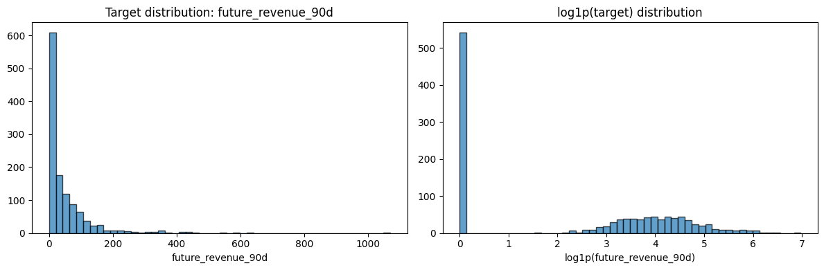
fig, axes = plt.subplots(1, 2, figsize=(12, 4))

axes[0].hist(final_dataset["future_revenue_90d"], bins=50, edgecolor="black", alpha=0.7)
axes[0].set_title("Target distribution: future_revenue_90d")
axes[0].set_xlabel("future_revenue_90d")

axes[1].hist(np.log1p(final_dataset["future_revenue_90d"]), bins=50, edgecolor="black", alpha=0.7)
axes[1].set_title("log1p(target) distribution")
axes[1].set_xlabel("log1p(future_revenue_90d)")

plt.tight_layout()
plt.show()

print("Target is right-skewed (common for revenue). log1p transform can be considered in downstream modeling.")

Target is right-skewed (common for revenue). log1p transform can be considered in downstream modeling.