Fallstudie: Vorhersage von Immobilienpreisen

Ziel dieser Fallstudie

• Anwendung der erlernten Methoden zur Vorhersage von Immobilienpreisen.

• Verwendung eines realen Datensatzes zur Modellierung.

• Umsetzung in Python mit scikit-learn.

Schritte zur Umsetzung

1. Daten laden und verstehen

   • Nutzung eines offenen Datensatzes (z.B. California Housing Dataset oder Kaggle Immobilienpreise).

   • Untersuchung der Datenverteilung, Korrelationen und möglicher Ausreißer.

2. Datenvorbereitung

   • Umwandlung kategorischer Merkmale (One-Hot-Encoding).

   • Normalisierung und Skalierung numerischer Merkmale.

   • Aufteilung in Trainings- und Testdaten.

3. Modelltraining mit Linearer Regression

   • Trainieren eines linearen Regressionsmodells mit scikit-learn.

   • Verwendung von Metriken zur Bewertung der Modellgüte (z.B. MSE, R²).

4. Modellbewertung und Interpretation

   • Bewertung der Modellperformance auf dem Testdatensatz.

   • Interpretation der wichtigsten Einflussgrößen.

Code-Beispiel

import sys
# !{sys.executable} -m pip install scikit-learn

Importe

import pandas as pd
import matplotlib.pyplot as plt
from sklearn.model_selection import train_test_split
from sklearn.preprocessing import StandardScaler
from sklearn.linear_model import LinearRegression
from sklearn.metrics import mean_squared_error, r2_score

Beispieldatensatz laden (California Housing Dataset)

from sklearn.datasets import fetch_california_housing

housing = fetch_california_housing()
df = pd.DataFrame(housing.data, columns=housing.feature_names)
df["PRICE"] = housing.target

df

	MedInc	HouseAge	AveRooms	AveBedrms	Population	AveOccup	Latitude	Longitude	PRICE
0	8.3252	41.0	6.984127	1.023810	322.0	2.555556	37.88	-122.23	4.526
1	8.3014	21.0	6.238137	0.971880	2401.0	2.109842	37.86	-122.22	3.585
2	7.2574	52.0	8.288136	1.073446	496.0	2.802260	37.85	-122.24	3.521
3	5.6431	52.0	5.817352	1.073059	558.0	2.547945	37.85	-122.25	3.413
4	3.8462	52.0	6.281853	1.081081	565.0	2.181467	37.85	-122.25	3.422
...	...	...	...	...	...	...	...	...	...
20635	1.5603	25.0	5.045455	1.133333	845.0	2.560606	39.48	-121.09	0.781
20636	2.5568	18.0	6.114035	1.315789	356.0	3.122807	39.49	-121.21	0.771
20637	1.7000	17.0	5.205543	1.120092	1007.0	2.325635	39.43	-121.22	0.923
20638	1.8672	18.0	5.329513	1.171920	741.0	2.123209	39.43	-121.32	0.847
20639	2.3886	16.0	5.254717	1.162264	1387.0	2.616981	39.37	-121.24	0.894

20640 rows × 9 columns

Aufteilung in Merkmale (x) und Zielvariable (y)

x = df.drop("PRICE", axis=1)
y = df["PRICE"]

Aufteilung in Trainings- und Testsets

x_train, x_test, y_train, y_test = train_test_split(
    x, y, test_size=0.2, random_state=42
)

Feature Scaling

scaler = StandardScaler()
x_train_scaled = scaler.fit_transform(x_train)
x_test_scaled = scaler.transform(x_test)

Lineare Regression trainieren

model = LinearRegression()
model.fit(x_train_scaled, y_train)

LinearRegression()

In a Jupyter environment, please rerun this cell to show the HTML representation or trust the notebook.
On GitHub, the HTML representation is unable to render, please try loading this page with nbviewer.org.

model.coef_

array([ 0.85438303,  0.12254624, -0.29441013,  0.33925949, -0.00230772,
       -0.0408291 , -0.89692888, -0.86984178])

model.intercept_

np.float64(2.071946937378881)

Vorhersagen treffen

y_pred = model.predict(x_test_scaled)

y_pred

array([0.71912284, 1.76401657, 2.70965883, ..., 4.46877017, 1.18751119,
       2.00940251], shape=(4128,))

Modellbewertung

mse = mean_squared_error(y_test, y_pred)
r2 = r2_score(y_test, y_pred)
print(f"Mittlerer quadratischer Fehler (MSE): {mse}")
print(f"Bestimmtheitsmaß (R²): {r2}")

Mittlerer quadratischer Fehler (MSE): 0.5558915986952444
Bestimmtheitsmaß (R²): 0.5757877060324508

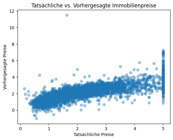
Visualisierung der Vorhersagen

plt.scatter(y_test, y_pred, alpha=0.4)
plt.xlabel("Tatsächliche Preise")
plt.ylabel("Vorhergesagte Preise")
plt.title("Tatsächliche vs. Vorhergesagte Immobilienpreise")
plt.show()